Customizing Excel
- By Bill Jelen
- 5/20/2022
- Performing a simple ribbon modification
- Adding a new ribbon tab
- Sharing customizations with others
- Questions about ribbon customization
- Using the Excel Options dialog box
- Options to consider
- Five Excel oddities
In this sample chapter fromMicrosoft Excel Inside Out (Office 2021 and Microsoft 365), you will walk through examples of customizing the Excel ribbon and learn about important option settings.
Performing a simple ribbon modification
Adding a new ribbon tab
Sharing customizations with others
Questions about ribbon customization
Using the Excel Options dialog box
Options to consider
Five Excel oddities
The Excel Options dialog box offers hundreds of changes you can make in Excel. This chapter walks you through examples of customizing the ribbon and discusses some of the important option settings available in Excel.
Performing a simple ribbon modification
Suppose that you generally like the ribbon, but there is one icon that seems to be missing. You can add icons to the ribbon to make it customized to your preference. If you feel the Data tab would be perfect with the addition of a pivot table icon, you can add it (see Figure 3.1).
)
Figure 3.1 Decide where the new command should go on the ribbon.
To add the pivot table command to the Data tab, follow these steps:
Right-click the ribbon and select Customize The Ribbon.
In the right list box, expand the Data tab by clicking the + sign next to Data.
Click the Sort & Filter entry in the right list box. The new group will go after this entry.
Click the New Group button at the bottom of the right list box. A New Group (Custom) item appears after Sort & Filter, as shown in Figure 3.2.
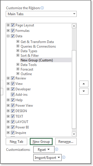
Figure 3.2 Commands must be added to a new group.
While the New Group is selected, click the Rename button at the bottom of the list box. The Rename dialog box appears.
The Rename dialog box offers to let you choose an icon and specify a name for the group. The icon is shown only when the Excel window is too small to display the whole group. Choose any icon and type a display name of Pivot. Click OK.
The left list box shows the popular commands. You could change Popular Commands to All Commands and scroll through 2,400 commands. However, in this case, the commands you want are on the Insert tab. Choose All Tabs from the top-left drop-down menu.
Expand the Insert tab, and then expand Tables. Click PivotTable in the left list box.
Click the Add button in the center of the dialog box to add PivotTable to the new custom Pivot group on the ribbon. Excel automatically advances to the next icon of Recommended PivotTables. Click Add again.
In the drop-down menu above the left list box, select All Commands. The left list box changes to show an alphabetical list of all commands.
Scroll through the left list box until you find PivotTable And PivotChart Wizard. This is the obscure entry point to create Multiple Consolidation Range pivot tables. Select that item in the left list box. Click Add. At this point, the right side of the dialog box should look like Figure 3.3.
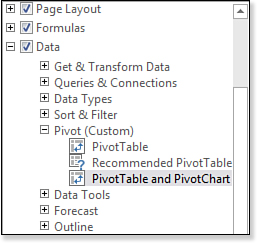
Figure 3.3 Three new icons have been added to a new custom group on the Data tab.
Click OK.
)
)
Figure 3.4 shows the new group in the Data tab of the ribbon.
)
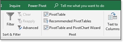
Figure 3.4 The results appear in the ribbon.