Customizing a pivot table

Formatting one cell is new in Microsoft 365

In the summer of 2018, a new trick appeared for Microsoft 365 customers. You can format a cell in a pivot table, and the formatting will follow that position.

For example, in Figure 3-37, a white font on dark fill has been applied to Revenue for Doodads sales to the Software sector.

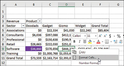
FIGURE 3-37 A new Format Cells option appears in the right-click context menu.

If you rearrange the pivot table, the dark formatting will follow the cell in the pivot table. While cell B9 was formatted in Figure 3-37, the formatting has moved to D5 in Figure 3-38.

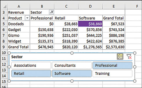
FIGURE 3-38 Rearrange the pivot table and the formatting moves so that revenue for Doodads sales to the Software sector stays formatted.

Note that the formatting will persist if you remove the cell due to a filter. If you unselect Software from the Slicer and then reselect Software, the formatting will return.

However, if you remove Sector, Product, or Revenue from the pivot table, the individual cell formatting will be lost.

In Figure 3-39, a Customer field has been added as the inner-row field. The dark formatting applied to Doodads sales of Software is now expanded to C5:C8 to encompass all four customers in this group. Note that in cell C9, the subtotal for Doodads sold to the Software sector is not formatted.

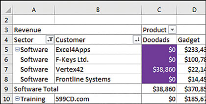
FIGURE 3-39 If you add an inner-row field, the formatting will expand to encompass all customers for Doodads in the Software sector.