Customizing a pivot table
- By Bill Jelen
- 1/10/2022
Although pivot tables provide an extremely fast way to summarize data, sometimes the pivot table defaults are not exactly what you need. In this sample chapter from Microsoft Excel Pivot Table Data Crunching (Office 2021 and Microsoft 365), you will learn how to make common cosmetic or report layout changes, add or remove subtotals, and change summary calculations.
In this chapter, you will:
Make common cosmetic changes
Make report layout changes
Customize a pivot table’s appearance with styles and themes
Change summary calculations
Change the calculation in a value field
Add and remove subtotals
Although pivot tables provide an extremely fast way to summarize data, sometimes the pivot table defaults are not exactly what you need. In such cases, you can use many powerful settings to tweak pivot tables. These tweaks range from making cosmetic changes to changing the underlying calculation used in the pivot table.
Many of the changes in this chapter can be customized for all future pivot tables using the new pivot table default settings. If you find yourself always making the same changes to a pivot table, consider making that change in the pivot table defaults.
In Excel, you find controls to customize a pivot table in myriad places: the PivotTable Analyze tab, Design tab, Field Settings dialog box, Data Field Settings dialog box, PivotTable Options dialog box, and context menus.
Rather than cover each set of controls sequentially, this chapter covers the following functional areas in making pivot table customizations:
Minor cosmetic changes—Change blanks to zeros, adjust the number format, and rename a field. If you find yourself making the same changes to each pivot table, see Tip 5: Use Pivot Table Defaults To Change Behavior Of All Future Pivot Tables in Chapter 14.
Layout changes—Compare three possible layouts, show/hide subtotals and totals, and repeat row labels.
Major cosmetic changes—Use pivot table styles to format a pivot table quickly.
Summary calculations—Change from Sum to Count, Min, Max, and more.
Advanced calculations—Use settings to show data as a running total, percent of total, rank, percent of parent item, and more.
Other options—Review some of the obscure options found throughout the Excel interface.
Making common cosmetic changes
You need to make a few changes to almost every pivot table to make it easier to understand and interpret. Figure 3-1 shows a typical pivot table. To create this pivot table, open the Chapter 3 data file. Select Insert, Pivot Table, OK. Select the Sector, Customer, and Revenue fields check boxes, and drag the Region field to the Columns area.
)
FIGURE 3-1 A typical pivot table before customization.
This default pivot table contains several annoying items that you might want to change quickly:
The default table style uses no gridlines, which makes it difficult to follow the rows and columns across and down.
Numbers in the Values area are in a general number format. There are no commas, currency symbols, and so on.
For sparse data sets, many blanks appear in the Values area. The blank cell in E5 indicates that there were no Associations sales in the Midwest. Most people prefer to see zeros instead of blanks.
Excel renames fields in the Values area with the unimaginative name Sum Of Revenue. You can change this name.
You can correct each of these annoyances with just a few mouse clicks. The following sections address each issue.
 Tip
Tip
Excel MVP Debra Dalgleish sells a Pivot Power Premium add-in that fixes most of the issues listed here. Debra’s add-in offers a few more features than the new PivotTable Defaults. This add-in is great if you will be creating pivot tables frequently. For more information, visit http://mrx.cl/pivpow16.
Applying a table style to restore gridlines
The default pivot table layout contains no gridlines and is rather plain. Fortunately, you can apply a table style. Any table style that you choose is better than the default.
Follow these steps to apply a table style:
Make sure that the active cell is in the pivot table.
From the ribbon, select the Design tab. Three arrows appear at the right side of the PivotTable Style gallery.
Click the bottom arrow to open the complete gallery, which is shown in Figure 3-2.
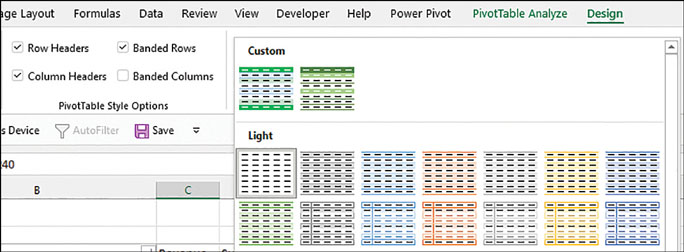
FIGURE 3-2 The gallery contains 85 styles to choose from.
Choose any style other than the first style from the drop-down menu. Styles toward the bottom of the gallery tend to have more formatting.
Select the check box for Banded Rows to the left of the PivotTable Styles gallery. This draws gridlines in light styles and adds row stripes in dark styles.
)
It does not matter which style you choose from the gallery; any of the 84 other styles are better than the default style.
 Note
Note
For more details about customizing styles, see “Customizing a pivot table’s appearance with styles and themes,” later in this chapter.
Changing the number format to add thousands separators
If you have gone to the trouble of formatting your underlying data, you might expect that the pivot table will capture some of this formatting. Unfortunately, it does not. Even if your underlying data fields were formatted with a certain numeric format, the default pivot table presents values formatted with a general format. As a sign of some progress, when you create pivot tables from Power Pivot, you can specify the number format for a field before creating the pivot table. This functionality has not come to regular pivot tables yet.
Note
For more about Power Pivot, read Chapter 10, “Unlocking features with the Data Model and Power Pivot.”
For example, in the figures in this chapter, the numbers are in the thousands or tens of thousands. At this level of sales, you would normally have a thousands separator and probably no decimal places. Although the original data had a numeric format applied, the pivot table routinely formats your numbers in an ugly general style.
What is the fastest way to change the number format? It depends if you have a single value field or multiple value fields.
In Figure 3-3, the pivot table Values area contains Revenue. There are many columns in the pivot table because Product is in the Columns area. In this case, right-click any number and choose Number Format.
)
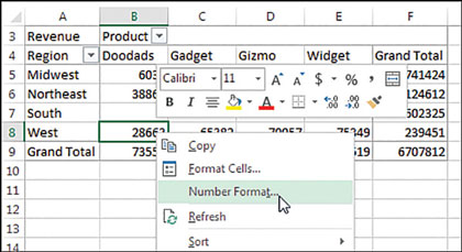
FIGURE 3-3 For a single value field, right-click any number and choose Number Format.
In contrast to Figure 3-3, the pivot table in Figure 3-4 contains three fields in the Values area: Revenue, Cost, and Profit. Rather than applying the Number Format to each individual column, you can format the entire pivot table by following these steps:
)
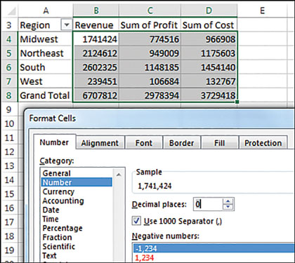
FIGURE 3-4 With multiple fields in the Values area, select all number cells as shown here and change the format using the Format Cells dialog box.
Select from the first numeric cell to the last numeric cell, including the Grand Total row or column if it is present.
Press Ctrl+1 to display the Format Cells dialog box.
Choose the Number tab across the top of the dialog box.
Select a number format.
Click OK.
Until a coding change in Excel 2010, the preceding steps would not change the number format in cases where the pivot table became taller. However, provided you include the Grand Total in your selection, these steps will change the number format for all the fields in the Values area.
Replacing blanks with zeros
One of the elements of good spreadsheet design is that you should never leave blank cells in a numeric section of a worksheet.
A blank tells you that there were no sales for a particular combination of labels. In the default view, an actual zero is used to indicate that there was activity, but the total sales were zero. This value might mean that a customer bought something and then returned it, resulting in net sales of zero. Although there are limited applications in which you need to differentiate between having no sales and having net zero sales, this seems rare. In 99% of the cases, you should fill in the blank cells with zeros.
Follow these steps to change this setting for the current pivot table:
Right-click any cell in the pivot table and choose PivotTable Options.
On the Layout & Format tab in the Format section, type 0 next to the field labeled For Empty Cells Show (see Figure 3-5). Alternatively, you can unselect the For Empty Cells Show option. Or, you can type anything here, such as a dash or even the words zip, nada, nothing.
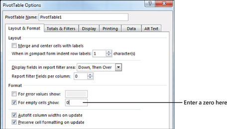
FIGURE 3-5 Enter a zero in the For Empty Cells Show box to replace the blank cells with zero.
Click OK to accept the change.
)
The result is that the pivot table is filled with zeros instead of blanks, as shown in Figure 3-6.
)
FIGURE 3-6 Your report is now a solid contiguous block of non-blank cells.
Changing a field name
Every field in a final pivot table has a name. Fields in the row, column, and filter areas inherit their names from the heading in the source data. Fields in the values section are given names such as Sum Of Revenue. In some instances, you might prefer to print a different name in the pivot table. You might prefer Total Revenue instead of the default name. In these situations, the capability to change your field names comes in quite handy.
Tip
Although many of the names are inherited from headings in the original data set, when your data is from an external data source, you might not have control over field names. In these cases, you might want to change the names of the fields as well.
To change a field name in the Values area, follow these steps:
Select a cell in the pivot table that contains the appropriate type of value. You might have a pivot table with both Sum Of Quantity and Sum Of Revenue in the Values area. Choose a cell that contains a Sum Of Revenue value.
Go to the PivotTable Analyze tab in the ribbon. A Pivot Field Name text box appears below the heading Active Field. The box currently contains Sum Of Revenue.
Type a new name in the box, as shown in Figure 3-7. Click a cell in your pivot table to complete the entry and have the heading in A3 change. The name of the field title in the Values area also changes to reflect the new name.
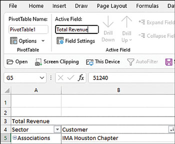
FIGURE 3-7 The name typed in the Custom Name box appears in the pivot table. Although names should be unique, you can trick Excel into accepting a name that’s similar to an existing name by adding a space to the end of it.
)
Tip
When you can see the value field name such as “Sum of Revenue” in the Excel worksheet, you can directly type a new value to rename the field. For example, in Figure 3-7, you could type Sales in cell A3 to rename the field.
Note
One common frustration occurs when you would like to rename Sum Of Revenue to Revenue. The problem is that this name is not allowed because it is not unique; you already have a Revenue field in the source data. To work around this limitation, you can name the field and add a space to the end of the name. Excel considers “Revenue ” (with a space) to be different from “Revenue” (with no space). Because this change is only cosmetic, the readers of your spreadsheet do not notice the space after the name.