Perform calculations on data

Create formulas to calculate values

After you add your data to a worksheet and define ranges to simplify data references, you can create a formula, which is an expression that performs calculations on your data. For example, you can calculate the total cost of a customer’s shipments, figure the average number of packages for all Wednesdays in the month of January, or find the highest and lowest daily package volumes for a week, month, or year.

To enter an Excel formula into a cell, you start with an equal (=) sign. Excel then knows that the expression that follows should be interpreted as a calculation, not text. After the equal sign, you enter the formula. For example, you can find the sum of the numbers in cells C2 and C3 by using the formula =C2+C3. After you have entered a formula into a cell, you can revise it by clicking the cell and then editing the formula in the formula bar. For example, you can change the preceding formula to =C3-C2, which calculates the difference between the contents of cells C2 and C3.

Entering the cell references for 15 or 20 cells in a calculation would be tedious, but in Excel you can easily enter complex calculations by using the Insert Function dialog box. The Insert Function dialog box includes a list of functions, or predefined formulas, from which you can choose.

Create formulas in the Insert Function dialog box.

The following table describes some of the most useful functions in the list.

Two other functions you might use are the NOW and PMT functions. The NOW function displays the time at which Excel updated the workbook’s formulas, so the value will change every time the workbook recalculates. The proper form for this function is =NOW(). You could, for example, use the NOW function to calculate the elapsed time from when you started a process to the present time.

The PMT function is a bit more complex. It calculates payments due on a loan, assuming a constant interest rate and constant payments. To perform its calculations, the PMT function requires an interest rate, the number of payments, and the starting balance. The elements to be entered into the function are called arguments and must be entered in a certain order. That order is written as PMT(rate, nper, pv, fv, type). The following table summarizes the arguments in the PMT function.

For example, if a company wanted to borrow $2,000,000 at a 6 percent interest rate and pay the loan back over 24 months, you could use the PMT function to figure out the monthly payments. In this case, you would write the function =PMT(6%/12, 24, 2000000), which calculates a monthly payment of $88,641.22.

You can also use the names of any ranges you have defined to supply values for a formula. For example, if the named range NortheastLastDay refers to cells C4:I4, you can calculate the average of cells C4:I4 with the formula =AVERAGE(NortheastLastDay).

With Excel, you can add functions, named ranges, and table references to your formulas more efficiently by using the application’s Formula AutoComplete capability. Just as AutoComplete offers to fill in a cell’s text value when Excel recognizes that the value you’re typing matches a previous entry, Formula AutoComplete offers to help you fill in a function, named range, or table reference while you create a formula.

As an example, consider a worksheet that contains a two-column Excel table named Exceptions. The first column is labeled Route; the second is labeled Count. You refer to the table by typing the table name, followed by the column or row name in brackets. For example, the table reference Exceptions[Count] would refer to the Count column in the Exceptions table.

Excel tables track data in a structured format.

To create a formula that finds the total number of exceptions by using the SUM function, you begin by typing =SU. When you enter the letter S, Formula AutoComplete lists functions that begin with the letter S; when you enter the letter U, it narrows the list down to the functions that start with the letters SU.

Excel displays Formula AutoComplete suggestions to help with formula creation.

To add the SUM function to the formula, click SUM and then press Tab. The function appears in the formula bar followed by an open parenthesis. To begin adding the table reference, enter the letter E. Excel displays a list of available functions, tables, and named ranges that start with the letter E. Click Exceptions, and press Tab to add the table reference to the formula. Then, because you want to summarize the values in the table’s Count column, enter an opening bracket, and, in the list of available table items, click Count. Finally, enter a closing bracket followed by a closing parenthesis to finish creating the formula =SUM(Exceptions[Count]).

If you want to include a series of contiguous cells in a formula, but you haven’t defined the cells as a named range, you can click the first cell in the range and drag to the last cell. If the cells aren’t contiguous, hold down the Ctrl key and select all the cells to be included. In both cases, when you release the mouse button, references to the cells you selected appear in the formula.

A SUM formula that adds individual cells instead of a continuous range.

In addition to using the Ctrl key to add cells to a selection, you can expand a selection by using a wide range of keyboard shortcuts. The following table summarizes many of these shortcuts.

After you create a formula, you can copy it and paste it into another cell. When you do, Excel changes the formula to work in the new cells. For instance, suppose you have a worksheet in which cell D8 contains the formula =SUM(C2:C6). If you click cell D8, copy the cell’s contents, and then paste the result into cell D16, Excel writes =SUM(C10:C14) into cell D16. In other words, it reinterprets the formula so it fits the surrounding cells! Excel knows to reinterpret the cells used in the formula because the formula uses a relative reference, or a reference that can change if the formula is copied to another cell. Relative references are written with just the cell row and column—for example, C14.

Relative references are useful when you summarize rows of data and want to use the same formula for each row. As an example, suppose you have a worksheet with two columns of data, labeled Sale Price and Rate, and you want to calculate a sales representative’s commission by multiplying the two values in a row. To calculate the commission for the first sale, you would enter the formula =A2*B2 in cell C2.

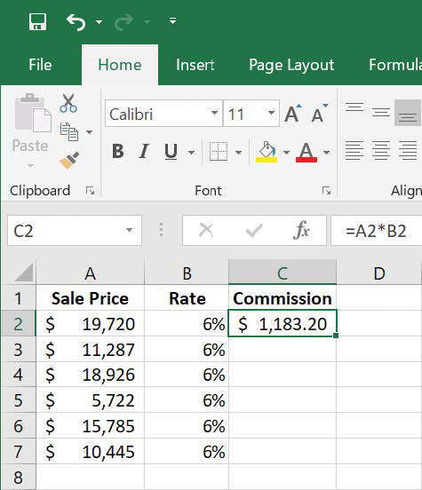
Use formulas to calculate values such as commissions.

Selecting cell C2 and dragging the fill handle until it covers cells C2:C7 copies the formula from cell C2 into each of the other cells. Because you created the formula by using relative references, Excel updates each cell’s formula to reflect its position relative to the starting cell (in this case, cell C2.) The formula in cell C7, for example, is =A7*B7.

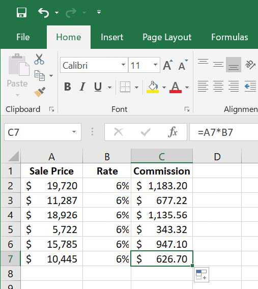
Copying formulas to other cells to summarize additional data.

You can use a similar technique when you add a formula to an Excel table column. For example, suppose the sale price and rate data were in an Excel table, and you created the formula =A2*B2 in cell C2. Excel would apply the formula to every other cell in the column. Because you used relative references in the formula, the formulas would change to reflect each cell’s distance from the original cell.

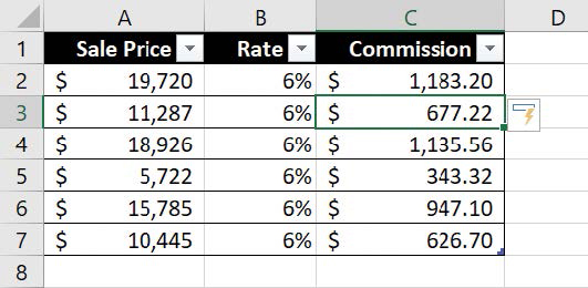
Adding a formula to an Excel table cell to calculate values in a column.

If you want a cell reference to remain constant when you copy the formula that is using it to another cell, you can use an absolute reference. To write a cell reference as an absolute reference, you enter $ before the row letter and the column number. For example, if you want the formula in cell D16 to show the sum of values in cells C10 through C14 regardless of the cell into which it is pasted, you can write the formula as =SUM($C$10:$C$14).

One quick way to change a cell reference from relative to absolute is to select the cell reference in the formula bar and then press F4. Pressing F4 cycles a cell reference through the four possible types of references:

• Relative columns and rows (for example, C4)

• Absolute columns and rows (for example, $C$4)

• Relative columns and absolute rows (for example, C$4)

• Absolute columns and relative rows (for example, $C4)

To create a formula by entering it in a cell

1. Click the cell in which you want to create the formula.

2. Enter an equal sign (=).

3. Enter the remainder of the formula, and then press Enter.

To create a formula by using the Insert Function dialog box

1. On the Formulas tab, in the Function Library group, click the Insert Function button.

2. Click the function you want to use in your formula.

   Or

   Search for the function you want, and then click it.

3. Click OK.

4. In the Function Arguments dialog box, enter the function’s arguments.

5. Click OK.

To display the current date and time by using a formula

1. Click the cell in which you want to display the current date and time.

2. Enter =NOW() into the cell.

3. Press Enter.

To update a NOW() formula

1. Press F9.

To calculate a payment by using a formula

1. Create a formula with the syntax =PMT(rate, nper, pv, fv, type), where:

   • rate is the interest rate, to be divided by 12 for a loan with monthly payments, by 4 for quarterly payments, and so on.

   • nper is the total number of payments for the loan.

   • pv is the amount loaned.

   • fv is the amount to be left over at the end of the payment cycle.

   • type is 0 or 1, indicating whether payments are made at the beginning or at the end of the month.

2. Press Enter.

To refer to a named range in a formula

1. Click the cell where you want to create the formula.

2. Enter = to start the formula.

3. Enter the name of the named range in the part of the formula where you want to use its values.

4. Complete the formula.

5. Press Enter.

To refer to an Excel table column in a formula

1. Click the cell where you want to create the formula.

2. Enter = to start the formula.

3. At the point in the formula where you want to include the table’s values, enter the name of the table.

   Or

   Use Formula AutoComplete to enter the table name.

4. Enter an opening bracket ([) followed by the column name.

   Or

   Enter [ and use Formula AutoComplete to enter the column name.

5. Enter ]) to close the table reference.

6. Press Enter.

To copy a formula without changing its cell references

1. Click the cell that contains the formula you want to copy.

2. Select the formula text in the formula bar.

3. Press Ctrl+C.

4. Click the cell where you want to paste the formula.

5. Press Ctrl+V.

6. Press Enter.

To move a formula without changing its cell references

1. Click the cell that contains the formula you want to copy.

2. Point to the edge of the cell you selected.

3. Drag the outline to the cell where you want to move the formula.

To copy a formula while changing its cell references

1. Click the cell that contains the formula you want to copy.

2. Press Ctrl+C.

3. Click the cell where you want to paste the formula.

4. Press Ctrl+V.

To create relative and absolute cell references

1. Enter a cell reference into a formula.

2. Click within the cell reference.

3. Enter a $ in front of a row or column reference you want to make absolute.

   Or

   Press F4 to advance through the four possible combinations of relative and absolute row and column references.