Perform calculations on data
- By Curtis Frye
- 4/9/2019
In this chapter form Microsoft Excel 2019 Step by Step, author Curtis Frye guides you through procedures related to streamlining references to groups of data on your worksheets and creating and correcting formulas that summarize an organization’s business operations.
Excel 2019 workbooks give you a handy place to store and organize your data, but you can do a lot more with your data in Excel than just store it. One important task you can perform is to calculate totals for values in a series of related cells. You can also use Excel to discover other information about data you select, such as the maximum or minimum value in a group of cells. And if you make an error, you can find the cause and correct it quickly.
Often, you can’t access the information you want without referencing more than one cell, and it’s also often true that you’ll use the data in the same group of cells for more than one calculation. Excel makes it easy to reference several cells at the same time, so you can define your calculations quickly.
This chapter guides you through procedures related to streamlining references to groups of data on your worksheets and creating and correcting formulas that summarize an organization’s business operations.
Name groups of data
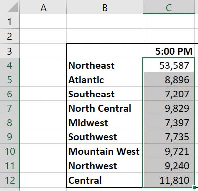
When you work with large amounts of data, it’s often useful to identify groups of cells that contain related data. For example, you can create a worksheet in which columns of cells contain data summarizing the number of packages handled during a specific time period and each row represents a region.
)
Instead of specifying the cells individually every time you want to use the data they contain, you can define those cells as a range (also called a named range). For example, you could group the hourly packages handled in the Northeast region shown in the preceding image into a group called NortheastVolume. Whenever you want to use the contents of that range in a calculation, you can use the name of the range instead of specifying the range’s address.
 TIP
TIP
Yes, you could just name the range Northeast, but if you use the range’s values in a formula in another worksheet, the more descriptive range name tells you and your colleagues exactly what data is used in the calculation.
If the cells you want to define as a named range have labels in a row or column that’s part of the cell group, you can use those labels as the names of the named ranges. For example, if your data appears in worksheet cells B4:I12 and the values in column B are the row labels, you can make each row its own named range.
Select a group of cells to create a named range.
If you want to manage the named ranges in your workbook—for example, to edit a range’s settings or delete a range you no longer need—you can do so in the Name Manager dialog box.
)
TIP
If your workbook contains a lot of named ranges, you can click the Filter button in the Name Manager dialog box and select a criterion to limit the names displayed in the dialog box.
To create a named range
Select the cells you want to include in the named range.
In the Name Box, next to the formula bar, enter a name for your named range.
Or
Select the cells you want to include in the named range.
On the Formulas tab of the ribbon, in the Defined Names group, click Define Name.
In the New Name dialog box, enter a name for the named range.
Verify that the named range includes the cells you want.
Click OK.
To create a series of named ranges from worksheet data with headings
Select the cells that contain the headings and data you want to include in the named ranges.
In the Defined Names group, click Create from Selection.
In the Create Names from Selection dialog box, select the check box next to the location of the heading text from which you want to create the range names.
Click OK.
To edit a named range
In the Defined Names group, click Name Manager.
Click the named range you want to edit.
In the Refers to box, change the cells to which the named range refers.
Or
Click Edit, edit the named range in the Edit Range box, and click OK.
Click Close.
To delete a named range
Click Name Manager.
Click the named range you want to delete.
Click Delete.
Click Close.