Basic Data Preparation Challenges

Using Column from Examples

Often, the first command you see on the left side of the ribbon can reveal the importance of a feature. That is why, for example, you can find PivotTable as the first command in the Insert tab of Excel. In the Power Query Editor, you can find one of the most important capabilities as the first command in Add Column tab. Column from Examples is a powerful feature that enables you to extract meaning from existing columns into a new column, without any preliminary knowledge of the different transformations available in the Power Query Editor.

By using Column from Examples, you can add new columns of data in the Power Query Editor by simply providing one or more sample values for your new column. When you provide these examples, Power Query tries to deduce the calculation needed to generate the values in the new column. This capability can be used as a shortcut to extract new meaning from data. This is a very powerful feature, especially for new users because it means you are not required to explore for the necessary transformation in the ribbons or memorize the M formulas to extract the meaningful data into the new column. If you simply provide a few examples in the new column, Power Query tries to do the work for you.

Exercise 2-3 provides a quick demonstration of Column from Examples with the dataset from Exercise 2-2.

Exercise 2-3, Part 1: Introducing Column from Examples

In Exercise 2-2, you learned how to split the product code into four elements. But imagine that you just need to extract the product size from the code. In this exercise you will learn how to do this by using Column from Examples.

If you didn’t follow Exercise 2-2, download the workbook C02E02.xlsx from https://aka.ms/DataPwrBIPivot/downloads and save it in the folder C:\Data\C02.

1. Start a new blank Excel workbook or a new Power BI Desktop report.

2. Follow these steps to import C02E02.xlsx to the Power Query Editor:

   1. In Excel: On the Data tab, select Get Data, From File, From Workbook.

      In Power BI Desktop: In the Get Data drop-down menu, select Excel.

   2. Select the file C02E02.xlsx and select Import.

   3. In the Navigator dialog box that opens, select Products and then select Edit.

3. In the Power Query Editor, you can now see in the Preview pane that the Product Number column contains four dash-separated codes (for example, VE-C304-S-BE). The challenge is to extract the third value, which reflects the size of the product.

   Select the Product Number column, and on the Add Column tab, select the Column from Examples drop-down menu, where you see two options:

   • From All Columns

   • From Selection

   In this exercise, you need to extract the size of the product from Product Number, so select From Selection.

   TIP

   In many cases, if you know in advance which columns should contribute to the new column, selecting the relevant input columns and then selecting From Selection in the Column from Examples drop-down menu will improve the chances that Power Query will provide a useful recommendation.

   The Power Query Editor now enters a new state. The Preview pane is pushed down, and a new section is shown on top of the Preview pane, with the message Enter Sample Values to Create a New Column. In the bottom-right part of this new section are OK and Cancel buttons to exit from this special state.

   On the right side of the Preview pane is an area with a new empty column. This is where you can enter your examples. Before you do so, rename Column1 to Size by double-clicking the header of the new column.

4. Double-click the first blank cell of the Size column in the Preview pane. A drop-down menu shows a few recommended examples that you can select from to create the new column. The values in the drop-down menu can provide some ideas of transformation that can be used to populate the new column.

5. In the first blank cell, enter S, which represents the bolded size value in the product number VE-C304-S-BE. Press Enter, and Power Query populates the new Size column with all the suggested values, as illustrated in Figure 2-6. Press Ctrl+Enter or click OK to create the column.

   

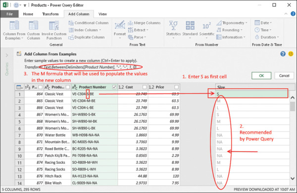
   FIGURE 2-6 The Power Query Editor in Add Column from Examples mode enables you to easily extract the size code from Product Number column.

6. You can now see the new Size column, calculated as expected. Load the data to your workbook or to a Power BI report and save.

You can download the solution files C02E03 - Solution.xlsx and C02E03 - Solution.pbix from https://aka.ms/DataPwrBIPivot/downloads.

Practical Use of Column from Examples

Column from Examples is a very useful tool to discover new transformations that are available in the user interface and in M. Let’s demonstrate how a new transformation can be discovered, using the output of Column from Examples. In step 6 of Exercise 2-3, Part 1, you can see that in the Applied Steps pane of the Power Query Editor, the last step, Inserted Text Between Delimiters, contains a settings control (in the shape of a cog) at the right side of the step. By clicking the settings control you can open the Text Between Delimiters dialog box. This dialog box allows you to extract text between delimiters. Now, when you know that such a dialog box exists, you can explore the Power Query Editor to find which ribbon command can trigger it, outside the Column from Examples flow. Exploring the Transform tab reveals the command Text Between Delimiters inside the Extract drop-down menu.

For intermediate Power Query users, a great way to improve knowledge of M is to use Column from Examples and review the suggested code that is shown in the top pane (highlighted in Figure 2-6). You may find some useful functions, such as Text.BetweenDelimiters, which is used in Exercise 2-3, Part 1.

Column from Examples can help you achieve a wide variety of transformations on text, dates, times, and numbers. You can even use it to create bucketing/ranges and conditional columns, as you will see in Exercise 2-3, Part 2.

Exercise 2-3, Part 2: Converting Size to Buckets/Ranges

In this part of Exercise 2-3, you will use Column from Examples to group numeric size values into buckets. You can download the solution files C02E03 - Solution.xlsx and C02E03 - Solution.pbix from https://aka.ms/DataPwrBIPivot/downloads to follow the steps of this exercise.

1. Open C02E03 - Solution.xlsx or C02E03 - Solution.pbix and launch the Power Query Editor. To launch the Power Query Editor in Excel, go to the Data tab, select Get Data, and then select Launch Power Query Editor. To launch the Power Query Editor in Power BI Desktop, select Edit Queries on the Home tab.

   You can see that the Size column contains a combination of alphabetic and numeric size values. In the next two steps you will learn how to ignore the textual values and focus only on numeric values in the Size column by creating a new column with the numeric representation for sizes. There are several ways to achieve this goal. In step 2, you will do it using the error-handling features in Power Query. In step 3, you will do it using Column from Examples.

2. To extract all the numeric sizes from the Size column by using error handling, follow these steps:

   1. Select the Size column. On the Add Column tab, select Duplicate Column.

   2. Rename the new column Size - Numbers and change its type to Whole Number by selecting the ABC control in the header and Whole Number in the drop-down menu.

   3. You now see Error values in all the cells that contained textual size codes (S, M, L, X, and NA), but you want to work on numbers only, so you need to replace the errors with nulls. To do this, select the Size - Numbers column, and on the Transform tab, select the Replace Values drop-down menu and then select Replace Errors. An easier way to find the Replace Errors transformation is by right-clicking on the column header and finding the transformation in the shortcut menu.

   4. In the Replace Errors dialog box that opens, enter null in the Value box and click OK to close the dialog box.

3. To extract the numeric size values by using Column from Examples, instead of replacing errors with null, follow these steps:

   1. If you applied step 2, delete the last four steps that were created in Applied Steps. Your last step should now be Inserted Text Between Delimiter.

   2. Select the Size column. On the Add Column tab, select the Column from Examples drop-down menu and then select From Selection.

   3. When the Add Column from Examples pane opens, showing the new column, rename it Size - Numbers.

   4. Double-click the first blank cell in the Size - Numbers column. You can see that the value in the Size column is S. Because you are not interested in textual size values, enter null in the first blank cell and press Enter.

   5. When you see that the second and third values in the Size column are M and L, enter null in both the second and third cells of Size - Numbers and press Enter.

   6. Move to the cell in row 7. You can see that the value in the Size column is NA. Enter null in the seventh cell of the Size - Numbers column and press Enter.

   7. Move to row 21. You can see that the value in the Size column is X. Enter null in the corresponding cell of the Size - Numbers column and press Enter.

   8. Now, in row 22, you see the value 60. Enter 60 in the corresponding cell of the Size - Numbers column and press Enter. Power Query populates the new Size column with all the suggested values. You can now press Ctrl+Enter to create the new Size - Numbers column.

   In Applied Steps, you can now see the new Added Conditional Column step. Select the settings icon or double-click this step, and the Add Conditional Column dialog box opens. This dialog box allows you to create a column based on conditions in other columns. You could also have reached this point, and created a new column for the numeric size values, by applying a conditional column instead of by using Column from Examples. Close the Add Conditional Column dialog box. You will learn about this dialog box In Exercise 2-4.

4. Change the type of the Size - Numbers column to Whole Number by selecting the ABC control in the header of the column in the Preview pane and Whole Number in the drop-down menu.

   In the next part of this exercise, you will create a separate table for the products with numeric sizes and will classify them into four size buckets (S = Small, M = Medium, L = Large, and X = Extra Large) by using Column from Example.

5. In the Queries pane, right-click Products and select Reference. Rename the new query Numeric-Size Products. To rename the query, right-click the query in the Queries pane and select Rename in the shortcut menu, or rename the query in the Query Settings pane, under Properties, in the Name box.

   TIP

   Using Reference is a very useful technique for branching from a source table and creating a new one, starting from the last step of the referenced query.

6. In the new query, remove all the products whose Size - Numbers value is null. To do so, click the filter control in the Size - Numbers column and select Remove Empty.

7. Say that you want to convert the numeric sizes into the buckets of X, L, M, and S as follows: Numbers equal to or greater than 70 will be assigned to the X bucket. Numbers equal to or greater than 60 will be assigned to L. Numbers equal to or greater than 50 will be assigned to M, and numbers equal to or greater than 40 will be assigned to S. Here are the steps to achieve this by using Column from Examples (see Figure 2-7 to ensure you follow the steps correctly):

   1. Select the Size - Numbers column, and in the Add Column tab, select the Column from Examples drop-down menu and then select From Selection.

   2. Rename the new column Size Bucket.

   3. Enter X in row 1 (because Size - Numbers is 70).

   4. Enter L in rows 2 and 3 (because the Size - Numbers values are 60 and 62, respectively).

   5. Enter M in row 5 (because Size - Numbers is 50).

   6. Enter S in row 20 (because Size - Numbers is 40).

   7. Press Ctrl+Enter to create the new Size - Bucket column. The Size - Bucket column now contains the required bucket names for the relevant ranges.

      

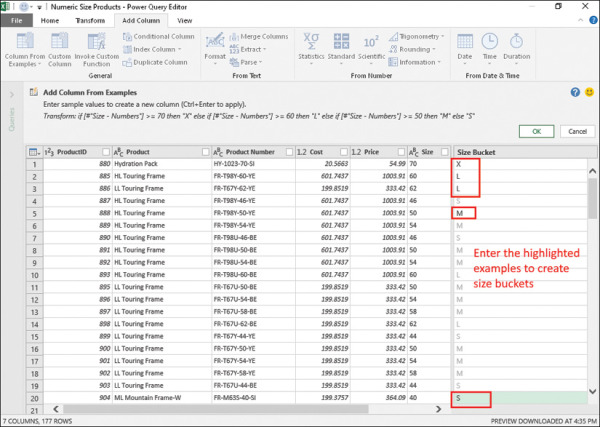
      FIGURE 2-7 You can use Add Column from Examples to create size buckets.

8. For learning purposes, double-click the Added Conditional Column step in the Applied Steps pane. The Add Conditional Column dialog box opens. Review the conditions that defined the ranges for each bucket, and close the dialog box.

9. Review the M formula in the formula bar for a quick glimpse into the M syntax, which is discussed in more detail throughout the book, specifically in Chapter 9, “Introduction to the Power Query M Formula Language.”

You can download the solution files C02E03 - Solution - Part 2.xlsx and C02E03 - Solution - Part 2.pbix from https://aka.ms/DataPwrBIPivot/downloads.