Basic Data Preparation Challenges
- By Gil Raviv
- 4/8/2019
- Extracting Meaning from Encoded Columns
- Using Column from Examples
- Extracting Information from Text Columns
- Handling Dates
- Preparing the Model
- Summary
In this sample chapter from Collect, Combine, and Transform Data Using Power Query in Excel and Power BI, author Gil Raiv introduces a variety of techniques in the Power Query Editor in Excel and Power BI for cleaning badly formatted datasets.
Before anything else, preparation is the key to success.
—Alexander Graham Bell
IN THIS CHAPTER, YOU WILL
Learn how to split and extract valuable information from delimiter-separated values
Learn how to enrich your data from lookup tables in a single table or by using relationships between fact tables and lookup tables
Learn how Add Column from Examples can help you extract or compute meaningful data from columns and use it to explore new transformations
Learn how to extract meaningful information, such as hyperlinks, from text columns
Handle inconsistent date values from one or more locales
Learn how to extract date or time elements from Date columns
Split a table into a fact table and a lookup table by using the Reference and Remove Duplicates commands
Learn how to avoid refresh failures when a lookup table contains duplicate values, even when you are sure you removed them
Split delimiter-separated values into rows to define group/member associations
Working with messy datasets can consume a lot of time for a data analyst. In the past, analysts needed to tackle badly formatted data with painful manual cleansing efforts. Excel power users could also use advanced formulas and VBA to clean and prepare data. Those who knew programming languages such as Python and R could harness their power to aid in the cleansing effort. But in many cases, data analysts eventually abandoned their exploration of messy datasets, uncertain of the return on investment they would get from cleaning the badly formatted data.
In this chapter, you will learn a wide variety of techniques in the Power Query Editor in Excel and Power BI for cleaning badly formatted datasets. These techniques will enable you to prepare your data in a matter of minutes. If you are new to Power Query, this chapter is the key to achieving a lot as a data analyst. The simple techniques that you will learn here will significantly reduce your data preparation time and enable you to tackle bigger challenges more quickly.
You may need to prepare messy data for an ad hoc analysis, or you might need to periodically prepare and circulate reports for large audiences. This chapter introduces the most common and basic data preparation techniques that will save your time and enable you to automate and streamline your efforts to gain insights.
Extracting Meaning from Encoded Columns
One of the most common challenges in unprepared data is to extract meaning from columns that are badly formatted. If you have a sequence of delimiter-separated codes or values in a single column, you might want to split them into multiple columns.
Excel provides native formula functions for extracting values from badly formatted text. You can use a combination of the functions LEFT, MID, RIGHT, FIND, SEARCH, and LEN to extract any substring from text. But often, the logic to extract the information you seek requires complex formulas and is hard to maintain over time, requiring you to expand the formulas to new rows when your source data changes.
The Text to Columns wizard in the Data tab of Excel enables you to easily split a column into multiple columns. Unfortunately, if you need to load a new table and apply the same type of split, you need to repeat the steps or use macros and VBA. In this section you will learn how you can use Power Query to tackle this challenge. You will find that the Power Query Editor in Excel and Power BI is extremely helpful, especially if you need to repeat the same tasks often, work with large datasets, or maintain a report over the long term.
AdventureWorks Challenge
In this chapter, you will work with the product catalog of a fictitious bike manufacturer company, AdventureWorks Cycles, in the AdventureWorks database.
Imagine that you are a new analyst in the fictitious company AdventureWorks. Your first task is to analyze the company’s product catalog and find out how many products the company manufactures by category, product size, and color. The list of products is provided in an Excel workbook that is manually exported from a legacy data warehouse. You can download the workbook C02E01.xlsx from https://aka.ms/DataPwrBIPivot/downloads.
Unfortunately, the product catalog is missing the Category, Size, and Color columns. Instead, it contains a Product Number, containing dash-separated values that include the information on category, size, and color. Figure 2-1 shows the mapping between the Product Number column and the missing columns.
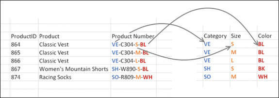
FIGURE 2-1 The AdventureWorks product catalog has category, size, and color values encoded inside the product number.
Your predecessor, who was recently promoted and now leads the Business Intelligence team, had solved this challenge by using Excel formulas. In the next exercise, you will learn how he implemented the solution.
Exercise 2-1: The Old Way: Using Excel Formulas
Download the workbook C02E01 - Solution.xlsx from https://aka.ms/DataPwrBIPivot/downloads. This workbook, which was implemented by your predecessor, uses Excel formulas to extract the product category, color, and size. In this exercise, you can follow his notes and learn how he implemented the solution—without using Power Query.
 NOTE
NOTE
Your goal in Exercise 2-1 is to review a typical solution in Excel, without using Power Query. You are not required to implement it or even fully understand it. As you will soon learn, the Power Query solution is simpler.
Open the workbook C02E01 - Solution.xlsx in Excel.
Review the first three worksheets: Products, Categories, and Colors. Products contains the main catalog table. In the Categories worksheet, you can see the mapping between category codes and values. For example, VE stands for vests, SH stands for shorts, WB stands for bottles, and BC stands for cages. In the Colors worksheet, you can see the mapping between color codes and values. For example, BE stands for blue, and BK stands for black.
The fourth worksheet contains three PivotTables with the kind of analysis you would expect to do. All the PivotTables are fed from the data in the Products worksheet.
In the Products worksheet, select the cell F2. In the formula bar, notice that this cell contains the following formula:
=LEFT(C2, 2)
The formula returns the two leftmost characters from column C, which contains the product number. These two characters represent the category code.
Select cell G2. In the formula bar, you can see the following formula:
=RIGHT(C2, 2)
The formula returns the two rightmost characters from column C, which contains the product number. These two characters represent the color code.
Select cell H2. In the formula bar you can see the following formula:
=SUBSTITUTE(MID(C2, SEARCH("-", C2, 8), 3), "-", "")This formula returns the code that represents the product size. This is where things become difficult. The inner formula searches for the character “-” in the product number at cell C2, starting from character 8. It returns the location of the character. Then, the MID function returns a three-digit substring. The substring may contain a leading or trailing dash character. The SUBSTITUTE function trims away the dash character.
Select cell I2. In the formula bar you can see the following formula:
=VLOOKUP(F2, Categories!A:B, 2, FALSE)
This formula returns the category value from the Categories worksheet, whose product code matches the value in F2.
Select cell J2. In the formula bar you can see the following formula:
=VLOOKUP(G2, Colors!A:B, 2, FALSE)
This formula returns the color value from the Colors worksheet, whose color code matches the value in G2.
If you are an Excel power user, it will not be difficult for you to implement the same formulas just described on a new dataset, such as in C02E01.xlsx. If you are not a power user, you can copy and paste the dataset from C02E01.xlsx to the relevant columns in the Products worksheet of C02E01 - Old Solution.xlsx, and then copy down all the formulas in columns F to J.
But what do you do if you need to update this workbook on a weekly basis? As you get constant product updates, you will need to perform a repetitive sequence of copies and pastes, which may lead to human errors and incorrect calculations. In the next two exercises, you will learn a better way to achieve your goals—by using Power Query.
Exercise 2-2, Part 1: The New Way
In this exercise, you will use the Power Query Editor to create a single Products table. Maintaining this new solution will be much easier than with C02E01 - Old Solution. A single refresh of the workbook will suffice, and you will no longer have many formulas in the spreadsheet to control and protect.
You can follow this exercise in Excel, Power BI Desktop, or any other product that includes the Power Query Editor.
Download the workbook C02E02.xlsx from https://aka.ms/DataPwrBIPivot/downloads and save it in a new folder: C:\Data\C02. The workbook contains the AdventureWorks database Products, Categories, and Colors worksheets. You will start the exercise by importing the three tables to the Power Query Editor.
Start a new blank Excel workbook or a new Power BI Desktop report.
Follow these steps to import C02E02.xlsx to the Power Query Editor:
In Excel: In the Data tab, select Get Data, From File, From Workbook.
NOTEDue to variations in the ribbons in the older versions of Excel, the instructions throughout the book from now on will assume you use Excel 2016 or later. (As a result, all entry points will be through the Get Data drop-down in the Data tab.) You can still follow these steps in the Power Query add-in for Excel 2010 and 2013 as well—the differences will be minuscule, and will only be applicable to the initial steps in the Data/Power Query ribbons. The ribbon differences among the Power Query versions is described in Chapter 1, “Introduction to Power Query,” in the section, “Where Can I Find Power Query?”
In Power BI Desktop: In the Get Data drop-down menu, select Excel.
Select the file C02E02.xlsx and select Import.
In the Navigator dialog box that opens in Excel, select the Select Multiple Items check box. In either Excel or Power BI Desktop, select the worksheets Categories, Colors, and Products and select Edit. (As explained in Chapter 1, If you don’t find the Edit button in the Navigator dialog box, select Transform Data, or the second button that is right to Load.)
In the Power Query Editor that opens, to the left you can see the Queries pane, which contains three queries—one for each of the worksheets you selected in the Navigator in step 2. By selecting each of the queries, you can see a preview of the data in the Preview pane. To the right, you can see the Query Settings pane and the Applied Steps pane, which shows you the sequence of transformation steps as you make changes to your query. Follow these steps to prepare the Categories and Colors queries:
In the Queries pane, select the Categories query. In the Preview pane, you will notice that the headers are Column1 and Column2. The first row contains the column names: Category Code and Product Category Name. To promote the first row, on the Transform tab, select Use First Row As Headers.
 TIP
TIPIf you prefer working with shortcut menus, you can click on the table icon in the top-left corner of the table in the Preview pane of the Power Query Editor and select Use First Row As Headers.
In the Queries pane, select the Colors query, which requires the same preparation step as the Categories query. Its column names are Column1 and Column2. The first row contains the actual column names, Color Code and Color. To promote the first row, on Transform tab, select Use First Row As Headers.
In the Queries pane, select the Products query.
Select the Product Code column either by clicking its header or by selecting the Choose Columns drop-down menu on the Home tab and then selecting Go to Column. When the Go to Column dialog box opens, select the Product Code column in the list and click OK to close the dialog box.
On the Transform tab, select Split Column and then select By Delimiter. You can also right-click the header of the Product Code column and select Split Column from the shortcut menu, and then select By Delimiter.
In the Split Column by Delimiter dialog box that opens, by default, the correct settings are selected, and you could simply click OK to close the dialog box, but before you do, review the elements of the dialog (see Figure 2-2):
The Custom option is selected in the dialog box, and the dash character is specified as a delimiter. This selection is recognized by Power Query because all the values in the columns are dash-separated.
Each Occurrence of the Delimiter is selected because there are multiple dash characters.
If you expand the Advanced Options section, you can see that Power Query detected that Product Number values can be split into four columns.
TIPWhen you have a fixed number of delimiters, the split into columns is effective. When you have an unknown number of delimiters, you should consider splitting the column into rows. Later in this exercise, you will learn when splitting into rows can be helpful.
You can see that the quote character is also set. Why do you need it? How will you split dash-separated values if one of the values contains a dash that should not be used as a delimiter? The owner of your data can use double quotes at the beginning and end of text that contains a dash. Power Query will not split the dash characters inside the quoted string. The only caveat is that when you have a double quote at the beginning of a value, but you are missing an ending double quote, the entire text starting from the double quote will be kept intact. To ignore quotes, select None as the quote character.
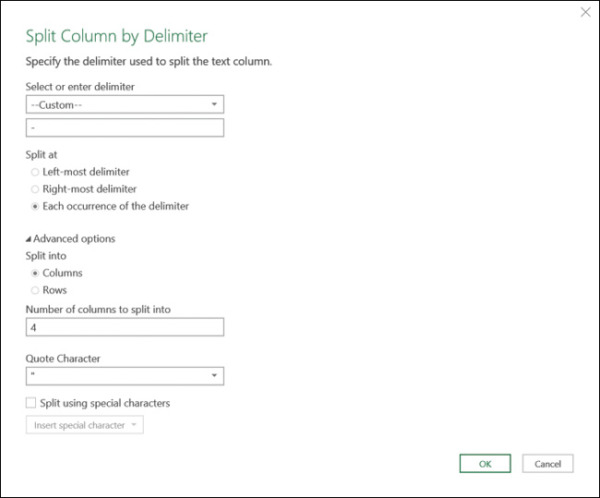
FIGURE 2-2 The Split Column by Delimiter dialog box is automatically set to split by the dash delimiter. More options can be found under Advanced Options. It is recommended that you review them and ensure that the default choices are correct.
After you close the Split Column by Delimiter dialog box, you can see in the Preview pane that the Product Number column is split into four columns: Product Number.1, Product Number.2, Product Number.3, and Product Number.4. Rename them Category Code, Short Product Number, Size, and Color. To rename a column, double-click the column name and type a new name. Alternatively, you can select the column and then select Rename in the Transform tab. The column name is then selected, and you can enter the new column name.
At this stage, you have extracted the size column, and you have separate codes for the product category and color. You will now learn two approaches for adding the actual category and color values instead of their codes. In Exercise 2-2, Part 2, you will learn how to merge the category and color values into the Products table, and in Exercise 2-2, Part 3, you will learn how to keep the three tables as fact and lookup tables.
To save the workbook or Power BI report follow these steps:
In Excel:
In the Home tab of the Power Query Editor, select the Close & Load drop-down menu and then select Close & Load To. The Import Data dialog box opens.
Select Only Create Connection and ensure that Add This Data to the Data Model is unselected. (In the third part of this exercise, you will select this check box.)
Save the workbook as C02E02 - Solution - Part 1.xlsx.
In Power BI Desktop: Select Close & Apply and save the report as C02E02 - Solution - Part 1.pbix.
)
Exercise 2-2, Part 2: Merging Lookup Tables
In this part of Exercise 2-2, you will merge the category and color values from the Categories and Colors queries into the Products query, according to their corresponding codes. Recall from Exercise 2-1 that mapping between the codes and the values can be done using VLOOKUP in Excel. In this exercise, you will learn an equivalent method using the Power Query Editor.
In Excel: Open the file C02E02 - Solution - Part 1.xlsx. In the Data tab, select Get Data and then select Launch Power Query Editor.
In Power BI Desktop: Open the file C02E02 - Solution - Part 1.pbix and select Edit Queries from the Home tab.
In the Power Query Editor that opens, in the Queries pane, select the Products query. On the Home tab, select Merge Queries.
In the Merge dialog box that opens, you can merge between two tables according to matching values in specified columns. You will merge the category names from the Categories query into the Products query, according to the matching category code. Figure 2-3 illustrates the following steps you need to take in the Merge dialog box:
Select the Category Code column in the Products table, and in the drop-down menu below the Products table, select Categories. Then select Category Code in the second table (refer to Figure 2-3).
In the Join Kind drop-down, make sure Left Outer (All from First, Matching from Second) is selected, and click OK.
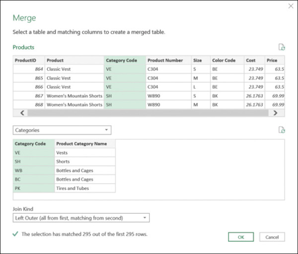
FIGURE 2-3 You can merge categories into products by category code in the Merge dialog box.
In the Power Query Editor, you can see that a new Categories column is added as the last column, with Table objects as values.
Expand the Categories column (by clicking on the control at the right side of its header or by selecting the Categories column, and then selecting Expand in the Transform tab).
In the Expand pane, deselect Category Code and deselect Use Original Column Name As Prefix. Then click OK. The new Categories column is transformed to a new column called Product Category Name, with the matching category values in each row.
Now that you have the actual category name, remove the Category Code column by selecting it and pressing the Delete key.
NOTEStep 6 may seem a bit awkward for new users, who are accustomed to Excel formulas. You may be surprised to find that Product Category Name remains intact after the removal of Category Code. But keep in mind that the Power Query Editor does not work like Excel. In step 3, you relied on Category Code, as you merged categories into products by using the matching values in the Category Code column. However, in step 6 you removed the Category Code column. Whereas a spreadsheet can be perceived as a single layer, Power Query exposes you to a multi-layered flow of transformations, or states. Each state can be perceived as a transitory layer or a table, whose sole purpose is to serve as the groundwork for the next layer.
To merge the colors into the Products query, on the Home tab, select Merge Queries again. When the Merge dialog box opens, follow these steps (see Figure 2-4):
Select the Color Code column in the Products table, and in the drop-down menu below the Products table, select Colors. Then select the Color Code column in the second table.
In the Join Kind drop-down, ensure that Left Outer (All from First, Matching from Second) is selected and click OK.
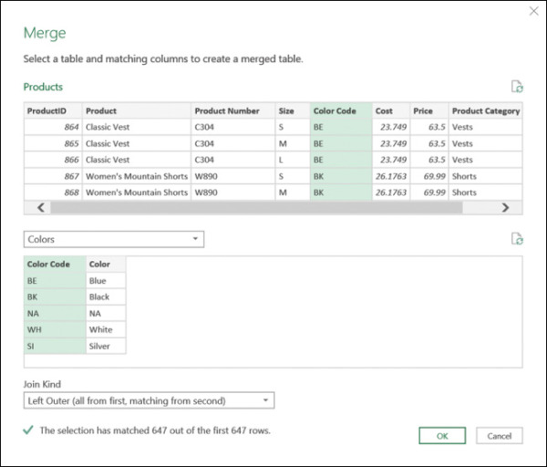
FIGURE 2-4 You can merge colors into products by color code in the Merge dialog box.
In the Power Query Editor, a new Colors column is added as the last column, with Table objects as values. Let’s pause for a moment and learn about the Table object and how to interact with it. In addition to the expand control located on the right side of the column, you have three common interactions with the Table objects:
You can drill down to a single Table object by clicking on any of the table hyperlinks. When you do so, a new step is added to Applied Steps, and from here you could potentially continue preparing your data, which is based on the selected Table object. Try it now.
Select any of the Table objects in the Colors column. The table in the Preview pane is transformed into a single-row table with the specific color code and color value that was merged in the cell that you selected. Delete this step from Applied Steps so you can get back to the Products table.
You can also drill down to a single Table object as a new query. This can allow you to explore the data of a single table, while keeping the original table intact. To drill down to a single Table object as a new query, right-click any of the Table objects and select Add As New Query. A new query is created, with all the transformation steps in Products, including the new drill-down step, which is equivalent to the drill-down in the preceding example. If you tried it, you can now delete the new query.
For temporary inspection of a specified table object, you can click on the space of any cell that contains a Table object. At the bottom of the Preview pane, you see a preview of the table. Now that you’ve learned a bit more about the Table objects, let’s expand the Colors column.
NOTEYou will find that working with other structured objects in the Power Query Editor—such as Record, List, and Binary objects—is similar: You can drill down to single object, add the object as a new query, or preview its content by clicking anywhere in the cell’s space.
Expand the Colors column (by clicking on the control at the right side of its header or by selecting the Colors column and then selecting Expand in the Transform tab).
In the Expand pane, deselect Color Code and deselect Use Original Column Name As Prefix. Then click OK. The new Colors column is transformed to Color, with the matching color values in each row.
Now that you have the actual color values, remove the Color Code column. The Products query is ready, and it’s time to load it to the report.
In Excel: Follow these steps to load Products into the Data Model:
In the Home tab of the Power Query Editor, select Close & Load.
In Excel, on the Data tab, select Queries and Connections to open the Queries pane. Right-click Products and select Load To.
In the Import Data dialog box that opens, select Add This Data to the Data Model and click OK.
You can now create a PivotTable that uses the Data Model and analyzes the distribution of colors or categories. On the Insert tab, select PivotTable. The Create PivotTable dialog box opens. Ensure that the option Use This Workbook’s Data Model is selected and click OK to close the dialog box.
In Power BI Desktop: Follow these steps:
In the Queries pane, right-click Categories and deselect the Enable Load check box.
Right-click the Colors query and deselect the Enable Load check box.
The last two steps allow you to treat specific queries as stepping-stones for other queries. Because you have extracted the category and color values from Categories and Colors, you can keep Products as the single table in your report. Deselecting Enable Load ensures that these queries are not loaded to the Power BI report. These steps are equivalent in Excel to step 9b, in Exercise 2-2, Part 1, where you selected Only Create Connection in the Import Data dialog box.
On the Home tab, select Close & Apply.
)
)
The Products table is now loaded and ready, with categories, colors, and sizes. To review the solution, including an example of a PivotTable with the distribution of products by color, download the workbook C02E02 - Solution - Part 2.xlsx from https://aka.ms/DataPwrBIPivot/downloads. To review the Power BI solution, download the report C02E02 - Solution - Part 2.pbix.
Exercise 2-2, Part 3: Fact and Lookup Tables
In Part 2 of Exercise 2-2, you merged the category and color values from the Categories and Colors queries into the Products query. While this approach enables you to have a single table with the necessary information for your report, there is a better way to do it, using relationships.
NOTE
When you import multiple tables, relationships between those tables may be necessary to accurately calculate results and display the correct information in your reports. The Excel Data Model (also known as Power Pivot) and Power BI Desktop make creating those relationships easy. To learn more about relationships in Power BI, see https://docs.microsoft.com/en-us/power-bi/desktop-create-and-manage-relationships.
In Part 3 of Exercise 2-2, you will start where you left off in Part 1 and load the three queries as separate tables in the Data Model.
In Excel: Open the file C02E02 - Solution - Part 1.xlsx. In the next steps you will load all the queries into the Data Model in Excel, which will enable you to create PivotTables and PivotCharts from multiple tables. On the Data tab, select Queries & Connections.
In the Queries & Connections pane that opens, right-click the Categories query and select Load To.
In the Import Data dialog box that opens, select Add This Data to the Data Model and close the dialog box.
Right-click the Colors query and select Load To.
In the Import Data dialog box that opens, select Add This Data to the Data Model and close the dialog box.
Right-click the Products query and select Load To.
In the Import Data dialog box that opens, select Add This Data to the Data Model and close the dialog box.
At this stage, you have the three tables loaded to the Data Model. It’s time to create the relationship between these tables.
On the Data tab, select Manage Data Model. The Power Pivot for Excel window opens.
On the Home tab, select the Diagram view.
In Power BI Desktop: Open the file C02E02 - Solution - Part 1.pbix and select the Relationships view from the left-side menu.
Drag and drop Category Code from the Categories table to Category Code in the Products table.
Drag and drop Color Code from the Colors table to Color Code in the Products table.
Your Data Model now consists of a fact table with the product list and two lookup tables with the supplementary information on categories and colors. As shown in Figure 2-5, there are one-to-many relationships between Category Code in the Categories table and Category Code in the Products table, as well as between Color Code in the Colors table and Color Code in the Products table.
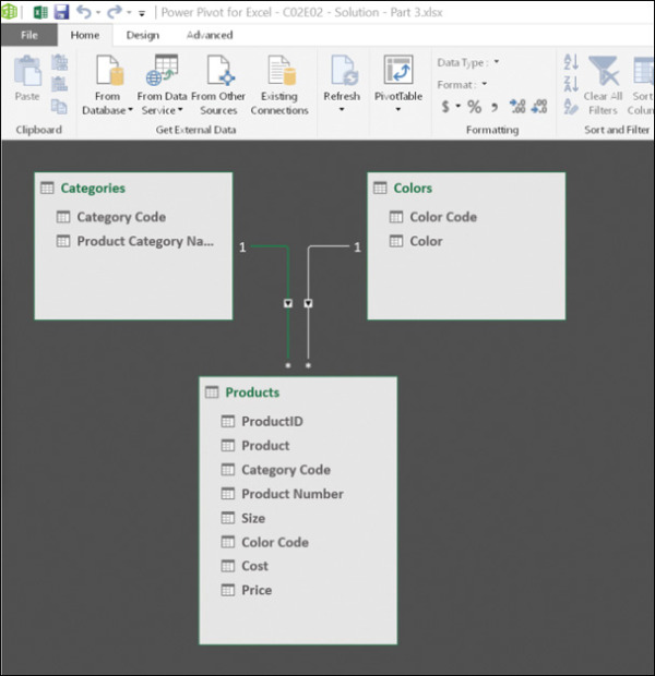
FIGURE 2-5 The Diagram view shows the Data Model relationships in Excel between Categories and Products and between Colors and Products.
After you have established the relationships between the tables, hide the columns Category Code and Color Code in the tables to ensure that these fields will no longer be selected in PivotTables, PivotCharts, and Power BI visualizations. By hiding these fields, you help report consumers enjoy a cleaner report. In other scenarios where you have multiple fact tables connected to a lookup table by the same column, hiding the column in the fact tables can lead to a more extendable report, in which a single column in the lookup table can be used in a slicer or a visual to filter data coming from the multiple fact tables.
In Excel, right-click Color Code in the Colors table and select Hide from Client Tools. Repeat this step on Color Code in the Products table and Category Code in the Categories and Products tables.
In Power BI, right-click Color Code in the Colors table and select Hide in Report View. Repeat this step on Color Code in the Products table and Category Code in the Categories and Products tables.
)
)
You can now create PivotTables, PivotCharts, and visualizations as demonstrated in the solution files C02E02 - Solution - Part 3.xlsx and C02E02 - Solution - Part 3.pbix, which are available at https://aka.ms/DataPwrBIPivot/downloads.
TIP
While the solution in Exercise 2-2, Part 2 simplifies your report, as it leaves you with a single table, in real-life reports that have multiple tables, the solution in Exercise 2-2, Part 3 will provide more opportunities for insight, as your model will become more complex. For example, having a single Categories lookup table connected to multiple fact tables with Product Category codes will allow you to compare between numerical columns across the different fact tables, using the shared categories.