Use other services for machine learning
- By Julio Granados and Ginger Grant
- 4/11/2018
- Skill 4.1: Build and use neural networks with the Microsoft Cognitive Toolkit
- Skill 4.2: Streamline development by using existing resources
- Skill 4.3: Perform data science at scale by using HDInsight
- Skill 4.4: Perform database analytics by using SQL Server R Services on Azure
- Thought experiment
- Thought experiment answers
- Chapter summary
Skill 4.3: Perform data science at scale by using HDInsight
This skill covers how to perform data science processes when your datasets are too big to fit in your typical development environment (e.g. your laptop) or Azure Machine Learning. On the other hand, maybe the type of data you are dealing with is too complex to be ingested with a regular tabular form and needs to be pre-treated with appropriate languages and storage platforms (e.g. big data technology) before you are able to create models on top of it.
Deploy the appropriate type of HDInsight cluster
HDInsight is the Microsoft cloud-based implementation of Hadoop clusters. It is offered as PaaS (Platform as a Service), giving you most of the common Hadoop Data Platform (HDP) services, such as HBase, Storm, or Spark, to name a few. When you create an HDInsight cluster, several VMs (either Windows or Linux) are provisioned and deployed, creating a connected and running cluster in around 20 minutes. The cluster is available worldwide, as any other PaaS resource in Azure.
You can use either Blob Storage Containers or Data Lake Storage accounts as the primary storage for your HDInsight cluster. Consequently, all data that you can access can be unstructured, semi-structured, or fully structured. You can delete the cluster if you are done using it, but the storage is available after the clusters deletion. Having computation (the cluster itself) detached from the storage (Blob Storage / Data Lake) allows you to have your clusters up and running only for the time you need them, destroying them when your data analyses are finished and thus save money. Depending on the services you need to use on top of your data you will create different cluster types, each of them with different price rates.
To create your HDInsight cluster you need to log into your Azure Portal and click New, and search HDInsight, and then Create. A step-by-step form appears. You will provide a cluster name, the type of the cluster, and the basic storage settings. In the example, basic security (user and password, both for administrative user and the secure connection –ssh- user) has been selected, although a private and public key could have been used if you had corporate keys and want to use certificates to connect securely. Note that you need to use a private and public key to connect from a local Visual Studio environment. As seen in Figure 4-26, you can select different cluster types.
)
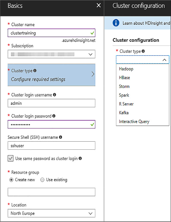
FIGURE 4-26 Initial HDInsight cluster configuration
The different types of clusters are based in the same structures, as described; supported at the time of writing this book are:
Hadoop The basic option uses HDFS, YARN, and Map Reduce programming models to process and analyze potentially massive and diverse data in a batch, parallel fashion. Tools like Hive for SQL-like queries are available in this mode.
HBase A NoSQL database on top of a traditional Hadoop cluster, providing strong consistency for large amounts of unstructured and semi-structured data.
Storm A distributed, real-time computation system for processing large streams of data. It is extremely scalable but requires manual implementation of its main elements, bolts, and spouts in Java or C# programming languages.
Spark A parallel processing framework that supports in-memory processing to boost big data analysis. Spark includes SQL-like, streaming data or machine learning applications that use the framework.
R Server A server for hosting and managing parallel, distributed R processes. It offers many improvements from the base R language with the ScaleR and other proprietary packages. It works both with Spark and with classic Hadoop jobs, acting as a “translator” of R scripts into Spark applications or Map Reduce jobs.
Kafka An open-source platform used for building streaming data pipelines and applications. It provides message-queue functionality, allowing you to publish and subscribe to data streams. It is often used along with Storm in the implementation of real-time event processing systems.
Interactive Query In-memory caching and improved columnar storage engine for Hive queries.
In this case, an R Server cluster is used so you will see examples and demos with it in the skill. Because R Server sits on top of a Spark cluster, all the features available in a Spark cluster are also available in an R Server cluster. R Server clusters include an extra node called Edge Node where the R Server engine resides, and the rest of the cluster is a normal Spark cluster. The Edge Node appears as “EN0” in Figure 4-27, where you can find the high-level architecture.
)
FIGURE 4-27 HDInsight Spark high-level architecture
The rest of the elements might be defined as follows:
HN - Head nodes Hadoop services under any HDInsight cluster type are installed and run in the head nodes. There are two head nodes to ensure high availability of these services. Therefore, head nodes control the access to the data and how computations are performed in the worker nodes.
WN - Worker nodes Worker nodes (also known as data nodes in different documentation) are the nodes that perform the computations on the data. They all can act in parallel to resolve a computation (sent by an application), or just some of them can be running an activity. They provide redundant access to the data.
GW - Gateway nodes By default each Spark cluster has two Gateway nodes for management and security. These nodes control access and management features as the Ambari Web UI or the SSH connections against the rest of the nodes in the cluster.
ZK - Zookeeper nodes Zookeeper nodes are used for leader election of master services on head nodes and to ensure that worker nodes and gateways know which head node has which master services running on. They are, in fact, responsible for availability and reliability of Hadoop clusters in HDInsight.
The election of the cluster type depends mainly on the type of workload you intend to perform with it. In this case, because you want to explore and build machine learning models on top of your datasets, either structured or unstructured, the ideal election seems to be R Server on Spark because both engines included have already been discussed. However, you can perform machine learning with other cluster configurations: only Spark using the MLlib, Spark with third-party applications like H2O machine learning, or classic Hadoop with Mahout to name a few. Even further, you might want to use other configurations like Hive on Hadoop to serve as big data repositories for other machine learning tools or libraries like Azure Machine Learning, as discussed in Chapter 1, “Prepare Data for Analysis in Azure Machine Learning.”
Once you have selected the type of cluster, you need to set up the storage settings. In the example, an Azure Storage account has been selected. That storage account holds the master and configuration data for you cluster. You can provide a secondary storage account to your cluster in order to access data from many sources. Different combinations are possible here: using an Azure storage account for your main data that you can reuse when creating a cluster on demand for data processing and accessing an Azure Data Lake Store as well as to consume data stored there.
You can also choose your metastore settings in case you want to preserve your metadata defined in Hive or Oozie (a workflow scheduler system to manage Hadoop jobs) between cluster creations when using a creation-processing-deletion schema. You can use an Azure SQL Database (even a very inexpensive one) to preserve that metadata to re-use it. Keep in mind that in Hive, for example, you create metadata to query your data, even if it is unstructured or semi-structured. These metadata collections might be complex and extensive, and some take a lot of time to develop. Consider saving this metadata if you do not want to lose all that development. For a complete example of storage options, see Figure 4-28.
)
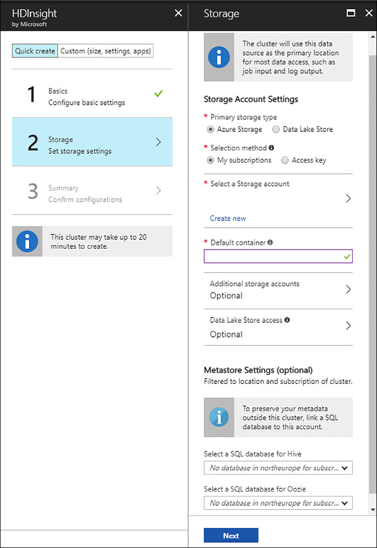
FIGURE 4-28 HDInsight Spark storage settings
For a detailed cluster creation process, click the Custom (Size, Setting, Apps) button in the main creation blade. In this custom mode you get to choose the third-party apps that you want to pre-install in your cluster, if it applies. In the example, at the moment of writing this book, there are no applications available for an R Server cluster on Linux. However, many applications are ready to pre-install in other types of clusters, easing the process to automatically provision an HDInsight cluster.
The next step is to choose among different sizes for your cluster’s nodes. Choosing the right size is not an easy task before you know your requisites: How big is your data? How fast will it grow? Which kinds of data science will you be tackling? Is the cluster going to be used to run other workloads beyond data science? Luckily, having HDInsight in Azure allows you to scale the number of worker nodes in a matter of minutes even when the cluster is already up and running, although some services might be restarted in the process. Note that you cannot change the sizes of the nodes once the cluster is created, neither the head nodes nor the workers. Therefore, sizing them appropriately is a key factor here. As a rule of thumb, increasing the size of head nodes increases the application serving capabilities of the cluster, while increasing the worker nodes sizes will allow us to run more jobs concurrently or to assign more resources to each job or query.
Consider that each Azure subscription has a limit in terms of cores that you can use, so the total number of cores in (including all the nodes in your cluster and other clusters that might exist in your subscription) cannot exceed that limit. However, you can ask for a higher limit contacting your subscription admin.
In the example shown in Figure 4-29, a two-worker node cluster is created with the default node sizes.
)
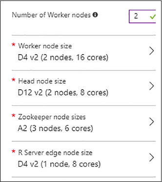
FIGURE 4-29 Node sizes
The fifth step in the creation process is to establish possible Script Actions and advanced networking options. In this example, this is not necessary, but keep in mind Script Actions if you need to install extra R packages in your nodes for your scripts. You will need to create a Script Action (one of the pre-configured existing ones) to set up such packages in your nodes, both edge and workers. You can also invoke custom bash (remember that you are working with Linux nodes in this case) scripts performing your own actions.
In the last step you see the summary of all your configurations before proceeding to create the cluster. Just click Create to provision your cluster.
Perform exploratory data analysis by using Spark SQL
As in any data science problem, an initial exploratory data analysis is fundamental to understanding your data and, at least having a basic comprehension of how much data is there, its distribution, and the relationships present between the features. By default, all HDInsight clusters come with sample data that you can use to test your applications or try different features on. In this example the Food Inspections dataset shows public restaurant inspections results from the city of Chicago.
Spark is a framework that allows you to process data and run applications in an in-memory fashion accessing the data stored in your HDInsight clusters. Many applications can run on top of that framework, leveraging the in-memory capabilities and the different programming languages available (natively, Java, Scala, and Python). These applications can be included in regular HDInsight Spark clusters, or are available to install as third-party applications.
One of these applications is Spark SQL, an engine that allows you to write SQL queries on top of in-memory data structures, which may come from many data sources. In the example, you access a CSV file present in the default Azure Storage Blob Container.
Once you have your HDInsight cluster already created you can write Spark SQL queries, for example, using a Jupyter Notebook running on top of Spark. You can access your list of Jupyter Notebooks on your HDInsight cluster clicking R Server Dashboards in your main cluster blade in the Azure Portal (see Figure 4.30).
)
FIGURE 4-30 R Server dashboards link
Once you have access to the reports, click the Jupyter Notebook button to launch the notebook tree (see Figure 4.31).
)
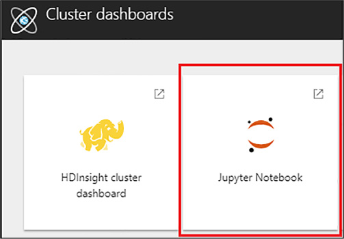
FIGURE 4-31 Jupyter Notebook trees link
You can access the same web UI using the URL: https://name_of_your_cluster.azurehdinsight.net/jupyter/tree. Here you see a list of existing Notebooks. To create a new Notebook, click the upper right button New and PySpark to create a Python notebook, as you did in Skill 1.2.
To start using the notebook and import the needed libraries from Spark SQL, you need a piece of code like the following:
from pyspark.sql import Row
from pyspark.sql.functions import UserDefinedFunction
from pyspark.sql.types import *
A Spark application is created automatically, as needed in any interaction with the Spark framework. You can use the sqlContext created automatically within the application to perform transformations on structured data as the CSV file that you will access, as well as many other libraries available in Python. See Figure 4-32 to see an example of a Spark application started.
)
FIGURE 4-32 Spark application started in a Jupyter Notebook
Your source data in this example is a CSV file. Therefore, you need to define a function that parses the data read from the raw text file. The results are stored in a Spark Resilient Distributed Dataset (RDD) because Spark SQL has not yet been invoked, and RDDs are Spark native data structure. You can use the “map” method, which is implemented by RDDs, to apply the function to the RDD returned by the “textFile” raw reader. You can find how in the following code:
def csvParser(s):
     import csv
     from StringIO import StringIO
     sio = StringIO(s)
     value = csv.reader(sio).next()
     sio.close()
     return value

# The sc variable is by default the name of the SparkContext, created when the Spark
application is initialized
restaurants = sc.textFile('wasb:///HdiSamples/HdiSamples/FoodInspectionData/Food_
Inspections1.csv').map(csvParse)
restaurants.take(1)
The output of this is the first row of the parsed CSV file stored in the RDD. As you can see in Figure 4-33, this row is not a header row because it is sometimes found in text files.
)
FIGURE 4-33 CSV file processed with a Python function in Spark
In order to process data with Spark SQL you need some structure in the dataset. Even when reading data from a CSV file (which is structured, although our data sources might be unstructured or semi-structured) you need to apply a schema to be able to process it with Spark SQL. You can do this in Python in Spark creating a Struct object and applying it using the lambda function. On top of that you can create a Spark SQL DataFrame, another type of object that allows you to write SQL queries using that object with the give schema. In the following code and in Figure 4-34 you see examples of this process.
#Define the struct object that will apply the desired schema
schema = StructType([
 StructField("name", StringType(), False),
 StructField("Type", StringType(), False),
 StructField("RiskLevel", StringType(), False),
 StructField("Date", StringType(), False),
 StructField("results", StringType(), False),
 StructField("violations", StringType(), True)])

#apply the lambda function and parse the output object into a Spark SQL dataframe
using the context
# As with the sc variable, sqlContext is created when the Spark session is
initialized
df = sqlContext.createDataFrame(restaurants.map(lambda l: (l[1], l[4], l[5],
l[10], l[12], l[13])) , schema)

#show the first 5 elements of the Spark SQL DataFrame
df.show(5)
)
FIGURE 4-34 Spark SQL DataFrame created and temporal table registered
You can even manipulate the data using other Python libraries like Pandas and custom defined functions. Pandas is a popular data structure manipulation open source library that might ease the manipulation process. In this example you go through a simple example but keep in mind that these custom defined functions might be invoking other more complex algorithms or libraries, enriching your dataset with little effort. Finally, you need to register the Spark SQL DataFrame as a temporary table in order to write SQL queries and visualize the results.
See the following code and Figure 4-35 for an example of this, counting the number of occurrences of the “pipe” character (|), and therefore retrieving the number of items in the text column called “violations” in the DataFrame shown in Figure 4-34.
import pandas as pd

def countViolations(st):
    number = len(st.split('|'))-1 #When no | is found, it would retrieve 1, so we
substract 1 by default
    return number

#cast the DataFrame into a Pandas data frame
df_pd = df.toPandas()

#create a new row applying the custom function
df_pd['numberOfViolations'] = df_pd['violations'].apply(countViolations)

#cast the object back into a Spark SQL DataFrame
df = sqlContext.createDataFrame(df_pd)

#register the DataFrame as a temporal table in Spark SQL
df.registerTempTable('restaurantsTable')

df.show(5)
)
FIGURE 4-35 Spark SQL DataFrame manipulated to add a column and registered as a temporal table
Now you can start writing SQL queries against the temporal table as if you were using a relational engine. Remember that, in fact, what you will be querying is an in-memory data object with a partial schema you applied in Figure 4-34 from a raw CSV file stored in an Azure Blob Storage account. The power behind that idea is that you are able to leverage your SQL knowledge to analyze data that is not purely structured; you are just applying a view of abstraction on top of it. Later in your analysis, you can apply many other data processing methods to get the most out of that data (a machine learning algorithm, for example).
In the following code and in Figure 4-36 you find how to query your temporal table, using the %%sql magic. Everything that will appear will be treated as SQL code, including the comments syntax.
%%sql

select Type, sum(numberOfViolations) as numberOfViolations
from restaurantsTable
group by Type
order by 2 desc
)
FIGURE 4-36 Spark SQL aggregated query
As you are executing this code in a Jupyter Notebook you can even create simple visualizations based on the results of your query. See Figure 4-37 for an example of visualizations using the results of other aggregated query, this time using the date field to see the evolution of the regulation violations over time using an area visualization, with its selector in the menu marked in red. Note that you can choose between aggregation functions, even when the Spark SQL query results already have an aggregation function.
)
FIGURE 4-37 Spark SQL query results represented by an area visual in the Jupyter Notebook
The Jupyter Notebook provides this visualization option, and it is useful for quick and easy analyses over data stored in Spark. However, going beyond you may be consuming Spark SQL query results from any data visualization tool with even better visual types and options and create analytic panels directly against your Spark SQL engine.
In this section, you have gone through some simple examples on how to create exploratory analysis over your data using Spark SQL, perhaps to continue creating more advanced analytics on top of such data. In the next section, you reuse the data already explored to learn how to build machine learning models in Spark.
Build and use machine learning models with Spark on HDI
After having explored and understood the dataset, and following the exact same experiment pipeline you have been following in the previous chapters, you are ready to start creating machine learning models within Spark on HDInsight. You can build them using libraries like MLlib, which is a Spark core library that offers machine learning features such as classification, regression, clustering, or Principal Component Analysis, among others.
In this section you learn how to create a classification model using the DataFrames you obtained up to Figure 4-10. Your goal is to predict the Risk Groups of the Chicago City inspections on different businesses based on their attributes or features. Note that the dataset you have been working on in the previous section has other fields that would fit as a label for a classification problem, even for a regression problem. This example intends to show the process itself, but changing just small pieces of code, you might obtain results for other labels as well.
)
You start evaluating the label you use, the RiskLevel column from your previously explored dataset. Spark SQL DataFrames (as well as other data manipulation libraries) have methods that you can leverage to get information that you might also obtain with other more classical languages, like any SQL ANSI-compliant one. For example, you subselect certain rows or columns from the DataFrame, apply filters, or transformations. In Figure 4-38 you find a distinct selection of the RiskLevel column.
)
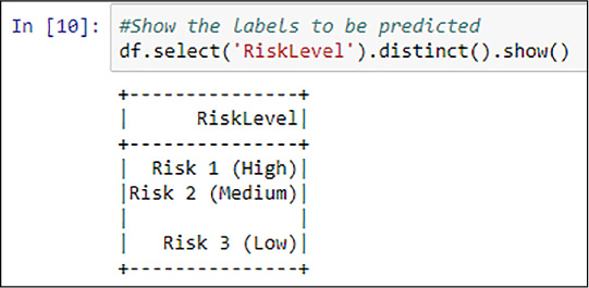
FIGURE 4-38 Spark SQL distinct RiskLevel values
Note that methods are used following each other, leveraging the objects retrieved by the previous operation. That is quite common in high-level programming languages like Python, and the concept of “pipeline of operations applied” is present in this example.
You might want to use the %%sql magic from the previously registered restaurantsTable temporal table to better understand how the distinct values are represented in the DataFrame. This is especially important since, as shown in Figure 4-38, there are blank values. The weight of such values in the dataset, as you have learned in Chapter 1, “Prepare Data for Analysis in Azure Machine Learning,” can be very important because it might undermine the importance of the useful (from the prediction perspective) values (Risks Low, Medium, and High). See Figure 4-39 for an example of an aggregated query studying the distribution of the RiskLabel values in the DataFrame.
)
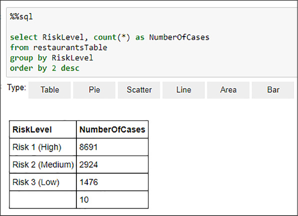
FIGURE 4-39 Spark SQL RiskLevel values distribution
From Figure 4-39 you can determine that the weight of the blank values in the distribution is not especially relevant. You treat this value appropriately in the next step. Now that you have understood the distribution of the data, you can start building a machine learning model using MLlib. For simplicity, you create a binary classification model.
Because, as seen in Figure 4-39, if the number of values of your label is higher than two, you need to transform these values into a binary form, represented by numbers in this case. You will divide the classes into High (coded as “1”) and Medium and Low (coded as 0). In order to do that, you can use the following code that implements a user defined function and creates a new dataset with the new label, the violations list, the type of the business, and the numberOfViolations columns that you created in Figure 4-35. See Figure 4-40 for an example of the execution.
# Import the necessary libraries for Spark SQL and Spark MLlib
from pyspark.sql import *
from pyspark.ml.feature import *
# Create a user defined function to code a binary label
def udf_createLabel(st):
    if st == 'Risk 1 (High)':
        return 1.0
    elif st == 'Risk 2 (Medium)' or st == 'Risk 3 (Low)':
        return 0.0
    else: #in case we are facing any other case, like blank spaces
        return 0.0

# Register the function as a UserDefinedFunction (function from the Spark SQL library)
returning a double data type
createLabel = UserDefinedFunction(udf_createLabel, DoubleType())

# Apply the UserDefinedFunction applying the 'label' alias, as well as the violations,
type and numberOfViolations fields
labeledData = df.select(createLabel(df.RiskLevel).alias('label'), df.violations,
df.Type, df.numberOfViolations)

labeledData.show(5)
)
FIGURE 4-40 Label creation using a user defined function in Spark SQL
You have created your binary risk label and your dataset already contains three feature columns. However, the Logistic Regression model that you use in MLlib only accepts DataFrames with a structure of label–vector of numeric features. Therefore, you need to transform your dataset to fit this structure.
First, you need to separate the violations column in words and apply a hashing function. This retrieves a column with the numeric representation of the text containing the violations committed by that particular business in the inspection. You can look at that representation as a codification of the text data, and therefore you can leverage the correlations between the number and type of violations committed, and the risk level.
You also need to transform the Type column into a numeric column. As mentioned, it is necessary that your feature vector is numeric to be fed to the Logistic Regression model. Luckily, MLlib provides a lot of tools and features, and one of them is a “string indexer” that you can use for this purpose.
Finally, you require the union of all these items you have up to this point: the hashed text feature, the Type column coded as a number, and the numberOfViolations feature that you previously had. Again, MLlib contains functionality for this with the VectorAssembler transformer.
In the following code sample you find all of these steps stored into objects in Spark. The goal of all these items is to use the previously processed data, referencing the new and / or transformed columns. That is why you will find references to columns that were not present yet but will be there when the transformers are invoked. You need all of these objects for the next step.
# Import needed MLlib libraries
from pyspark.ml import Pipeline
from pyspark.ml.classification import LogisticRegression
from pyspark.ml.feature import HashingTF, Tokenizer

# Definition of each stage of the pipeline to process the DataFrame
# Tokenizer for the text column dividing the text attribute in a new vector of
words
tokenizer = Tokenizer(inputCol="violations", outputCol="words")

# Hashing stage to create a vector of numeric features representing the text
features from the tokenizer
hashingTF = HashingTF(inputCol=tokenizer.getOutputCol(), outputCol="feats")

# String indexer to convert the Type string column into numeric values. Logistic
regression in MLlib only accepts numeric features
strIndexer = StringIndexer(inputCol="Type", outputCol = "TypeID")
strIndexer.setHandleInvalid("skip")

# Transformation to assemble all the vectors into a final single vector to feed
the Logistic Regressor
assembler = VectorAssembler(inputCols=["feats", "TypeID", "numberOfViolations"],
outputCol = "features")
Now that you have all the transformers in place, you are ready to build your Logistic Regression model. In order to do that, you use the MLlib Pipeline object, used to chain multiple transformer objects (as the ones you created in the previous piece of code). At the end of this pipeline you will place your Logistic Regression model, which will consume the processed data (remember, in a form of label – vector of features) and will be trained.
# Creation of the Logistic regression model
lr = LogisticRegression(maxIter=10, regParam=0.01)

# Creation of the pipeline with the different stages (from left to right), finally using
the logistic regression model fed with the processed data
pipeline = Pipeline(stages=[tokenizer, hashingTF, strIndexer, assembler, lr])

#Fit the pipeline sequence, retrieving the final model trained with the processed
dataframe
model = pipeline.fit(labeledData)
A few seconds after you run this code, your Logistic Regression model is trained and stored in your model object.
Now is time to test its performance. In your HDInsight sample folders there is another Food Inspections CSV file. You need to pre-process it in the same way you did with the first dataset. However, to create the predictions using that data you will not need to re-execute the Pipeline you created for the test data. Instead of this, you only need to call the function transform from the model you have trained and it will apply the same transformations that were applied to the original data, which is required for the building of the model. Remember from Chapter 2 that your test dataset should have the same schema as your training dataset for the algorithm to be able to create predictions. See Figure 4-41 for the result of the execution of this code.
#Load test data to predict using the model
testData = sc.textFile('wasb:///HdiSamples/HdiSamples/FoodInspectionData/Food_
Inspections2.csv')
.map(csvParse)

# Apply the lambda function and parse the output object into a Spark SQL dataframe
using the context
df_test = sqlContext.createDataFrame(testData.map(lambda l: (l[1], l[4], l[5], l[10],
 l[12], l[13])) , schema)

# Cast the DataFrame into a Pandas data frame
df_test_pd = df_test.toPandas()

# Create a new row applying the custom function
df_test_pd['numberOfViolations'] = df_test_pd['violations'].apply(countViolations)

# Cast the object back into a Spark SQL DataFrame
df_test = sqlContext.createDataFrame(df_test_pd)

# Apply the UserDefinedFunction applying the 'label' alias, as well as the violations,
 type and numberOfViolations fields
df_test = df_test.select(createLabel(df_test.RiskLevel).alias('label'),
df_test.violations, df_test.Type, df_test.numberOfViolations)

# Apply the transformations needed to fit the model's schema and create predictions on
test data
predictionsDF = model.transform(df_test)

predictionsDF.printSchema()
)
FIGURE 4-41 Test data preprocessing and prediction creation using MLlib
If you want to test the performance of the model on your test dataset, you need to compare the already observed label and the predictions. From the schema in Figure 4-41 you can infer that these columns are called label and prediction. In the following code sample you create a simplified DataFrame. and from it, register a temporal table to analyze the results with familiar SQL code using Spark SQL again.
simpleDF = predictionsDF.select(predictionsDF.label, predictionsDF.prediction)
simpleDF.registerTempTable('Preds')
Now, you are able to use your existing SQL skills to test the performance of your model. Use the following sample code for that purpose and see Figure 4-42 for the results.
%%sql

select
cast(sum(case when (label = 1.0 and prediction = 1.0) or (label = 0.0 and prediction
 = 0.0) then 1 else 0 end) as double) as NumberOfSuccesses,
cast(sum(case when (label = 1.0 and prediction = 1.0) or (label = 0.0 and prediction
 = 0.0) then 0 else 1 end) as double) as NumberOfFailures,
count(*) as TotalCases,
(cast(sum(case when (label = 1.0 and prediction = 1.0) or (label = 0.0 and prediction
 = 0.0) then 1 else 0 end) as double) / count(*)) * 100 as Accuracy
from Preds
)
FIGURE 4-42 Model performance evaluation using Spark SQL
With a measured accuracy of nearly 69 percent your model is showing a good (although improvable) performance. You can even create a more detailed visual analysis adding the True Positive, True Negative, False Positive, and False Negative classification you already learn in Chapter 2 Develop Machine Learning Models. Follow the next sample code and see Figure 4-43 for the detailed performance results.
%%sql

Select case
    when label = 1.0 and prediction = 1.0 then 'True Positive'
    when label = 0.0 and prediction = 0.0 then 'True Negative'
    when label = 0.0 and prediction = 1.0 then 'False Positive'
    when label = 1.0 and prediction = 0.0 then 'False Negatives'
    else 'Unknown' end as Cases
from Preds
)
FIGURE 4-43 Model performance evaluation using Spark SQL and Jupyter visualizations
In this section, you have reviewed how to manipulate Spark SQL DataFrames and the construction of pipelines with Spark MLlib to train and consume machine learning models. The use of an in-memory framework like Spark with support for high-level languages and exploration tools like Jupyter Notebooks allows you to rapidly create an end-to-end machine learning experiment. You could easily transform the code in your Notebooks to create Python or Scala scripts to train and / or consume your machine learning models on a scheduled basis, depending on your business requirements.
Build and use machine learning models using MapReduce
MapReduce is a data processing technique that allows parallel computations on clusters. Using this programming model it is possible to process large amounts of data in a batch fashion, even reaching petabytes of data. MapReduce breaks down into two phases:
Map Each working node receives a subset of the data and transforms it into (key, value) tuples.
Reduce Tuples with the same key are sent to the same node and it applies a reduction function.
A popular open source implementation of this programming model is the one included in HDInsight clusters. In this section, you learn to create a recommendation system for movies using Mahout (similar to the one created in Chapter 3, “Operationalize and Manage Azure Machine Learning Services”). Mahout is a framework for building scalable machine learning algorithms on top of clusters. To achieve this scalability, Mahout algorithms are implemented using MapReduce to fetch, process, and retrieve the data they use.
For this example you can use the same cluster you have used so far in this chapter. The data used for this example is sample data that is copied to blob storage when the cluster is deployed. We launch the recommendations using SSH, so the first step is to open an SSH connection with the cluster.
The files you use are located in the blob storage in the /HdiSamples/HdiSamples/MahoutMovieData/moviedb directory. The moviedb.txt file contains a list of movies in movieID|title|… format. You only use the first two columns (movieID and title) as a lookup table in order to transform the movies IDs returned by the recommender into titles. The file user-ratings.txt has a structure of userID, movieID, userRating, and timestamp. Mahout will use this file as training data. The file contains scores of 100 users, so it is an example file and you cannot expect to get good recommendations with so little data. After executing the recommendation, 10 recommendations per user are obtained.
hdfs dfs -text /HdiSamples/HdiSamples/MahoutMovieData/moviedb.txt
hdfs dfs -text /HdiSamples/HdiSamples/MahoutMovieData/user-ratings.txt
Run the recommendation with the command below. In addition to specifying the file with the input data (-i option), where to save the output data (-o), and where to save the temporary files (--tempDir), you can provide the similarity function used during model training (-s). With this command, Mahout launches MapReduce jobs that will read input data and train the model in parallel. When the model is trained, it calculates which 10 films are recommended for each user and saves the results in a file. The output file generated can be consumed in many ways, but in this example you will use Spark to transform and display the data.
mahout recommenditembased -s SIMILARITY_COOCCURRENCE -i /HdiSamples/HdiSamples/
MahoutMovieData/user-ratings.txt -o /example/data/mahoutout --tempDir /temp/mahouttemp
Many log messages appear in the console until the program is finished (see Figure 4-44).
)
FIGURE 4-44 Running Mahout item based recommender system
The output is saved on the file /example/data/mahoutout/part-r-00000 (output directory indicated by the option -o of the Mahout command).
hdfs dfs -text /example/data/mahoutout/part-r-00000
)
FIGURE 4-45 First lines of the output file
The fist column is the user id and the second column contains a list of movieID:recommendationScore ordered by recommendation score. In order to interpret these results correctly, further processing is necessary. In this example, you are going to use Spark for reading the output and the moviedb.txt files, and replace the movie IDs with the movie title. Open a new Jupyter Notebook and paste the following code in the first cell:
from pyspark.sql.functions import explode

def moviesParser(line):
    movie_id, title = line.split("|")[0:2]
    return movie_id, title

def recommendationsParser(line):
    user_id, recom = line.split("\t")
    # List of IDs of the recommended movies, ignoring predicted score
    recom = [i.split(":")[0] for i in recom.strip("[]\n").split(",")]
    return user_id, recom

# Set loaders and parsers
movies = sc.textFile('wasb:////HdiSamples/HdiSamples/MahoutMovieData/moviedb.
txt').map
(moviesParser).toDF()
recommendations = sc.textFile('wasb:///example/data/mahoutout/part-r
-00000').map(recommendationsParser).toDF()

# Create dataframes
movies_df = movies.toDF("movie_id", "title")
recommendations_df = recommendations.toDF("user_id", "movie_id")
# Recommendations array to rows
recommendations_df = recommendations_df.withColumn("movie_id",
 explode(recommendations_df.movie_id))
This code reads both files from the HDFS locations and saves the data in Spark DataFrames. For the recommendations DataFrame another step is performed: the recommendation array is unrolled in rows. Thus, if the arrays contain 10 recommendations per user, there will be 10 rows per user.
If you want, you can visualize the data using the show method of the DataFrames (see Figure 4-46).
)
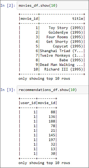
FIGURE 4-46 Fist 10 lines of the loaded DataFrames
The only thing left to do is to filter the recommendations of a specific user, join the two dataframes by movie_id, and show the results. This is what the following code does, and the output is shown in Figure 4-47.
def printUserRecommendations(id):
    recommendations_df.where("user_id == {}".format(id))        .join(movies_df, recommendations_df.movie_id == movies_df.movie_id)        .select("user_id", "title")        .show(10, False)

# Show recomendations of user 3
printUserRecommendations(3)
)
FIGURE 4-47 Recommendations of the user with id 3
Notice that Mahout does not delete temporary data that is created while processing the jobs, so you need to do it manually. Use the next command for deleting the output folder (indicated by the option --tempDir when calling the Mahout command):
hdfs dfs -rm -f -r /temp/mahouttemp
MapReduce is good for large-scale data processing, but unlike Spark, it does not load the data into memory and keeps it in a cache. MapReduce relies on disk. This is a problem in iterative processes where you have to access disk in each iteration to reload the same data, thus becoming a bottleneck. As you know, machine learning algorithms are iterative processes, so training models with MapReduce is much less efficient than using other approaches like Spark. A Spark implementation of machine learning algorithms can be up to 10 times faster than using MapReduce.
Build and use machine learning models using Microsoft R Server
Historically, the use of R in the machine learning industry has been burdened by three main weaknesses of the language itself:
Single-threaded processing
Memory limitation
Need to move data around in inefficient formats (mainly text files)
In the modern data analytics ecosystem, with ever-growing data amounts and some companies, like Revolution Analytics, started to develop frameworks and tools to overcome these limitations. These tools and frameworks work with Big Data platforms seamlessly, liberating the data scientists of the burden of having to write their own MapReduce jobs or learning other languages, leveraging their expertise and keeping their productivity while taking advantage of massive amounts of data and big clusters.
Microsoft bought Revolution Analytics in May 2015, absorbing and incorporating its technology into new products rapidly. From that acquisition and further developments, Microsoft has formed an R-based stack offering. Its enterprise-grade product, R Server, is 100 percent compatible with base R and offers multiple enhancements, such as:
Parallel algorithms
Compressed native data format
Data chunking to overcome memory limitations
In-database machine learning analytics
R Server can be used as a standalone product (either in a single machine or as a farm), inside SQL Server with ML Services (see Skill 4.4), or on top of a Spark HDInsight cluster. R Server appears as another R distribution if you are using it in a standalone or inside SQL Server. Therefore, you are able to use it from any IDE you want (e.g. Visual Studio, R Studio, R GUI, etc.).
In this example you go through an example using R code from a local Visual Studio 2017 IDE with R Tools installed (you can find them at https://www.visualstudio.com/vs/rtvs/) using the R Server cluster created at the beginning of this skill (Figures 4-1 to 4-4). You will be using the NYC Yellow Taxi Trip Data (available at http://www.nyc.gov/html/tlc/html/about/trip_record_data.shtml). The combination of these CSV files stores around 173 million rows and occupies 27GB uncompressed. For the sake of the example, only year 2013 is considered, but you can add other years for your own purposes.
)
)
R Server is able to use different compute contexts with minimal code changes. Compute contexts are a representation of where and how computations will be performed. For example, if your compute context is set to your local environment, R Server will understand that all operations over files will be computed using local CPUs, a local file system (whatever the operating system that you are using, R Server works in Windows and Linux) and that there is no cluster structure to take in account. When using a Spark compute context, all these assumptions will be different, and R Server adapts its internal algorithms to the new context.
In order to create the compute context, you need to use the rxSparkConnect clause. With a sample code like the following, you specify the different parameters of your Spark compute context, and a Spark application will be created if the resources you are asking for (worker nodes, memory allocations, and cores per executor) are available. YARN takes care of this. To connect from Visual Studio (or R Studio) you need several items:
Your cluster to have been created using a public certificate for the sshuser authentication (see Figure 4-48). You can create a public-private certificate using PuTTYgen (see how at https://www1.psfc.mit.edu/computers/cluster/putty.html).
)
The name of the edge node where the R Server engine resides. It will always have the following structure “yourClusterName-ed-ssh.azurehdinsight.net.”
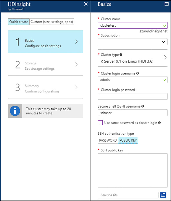
FIGURE 4-48 R Server cluster creation with Public Key for SSH user
## Spark context configuration
numberOfWorkerNodes <- 2 # number of worker nodes in cluster
executorCores <- 8 # cores of each executor. In this case, cores of each worker
node
myNameNode <- rxGetOption("hdfsHost")

## Private key has to be created without comment (a space is created in the whole
name and is not supported)
mySshUsername <- "sshuser"
mySshHostname <- "the_edge_node_url_of_your_cluster" #public facing cluster IP
address
mySshSwitches <- "-i your_private_key" #use .ppk file with PuTTY
mySshClientDir <- "C:/Program Files/PuTTY" #your path to PuTTY
myShareDir <- paste("/var/RevoShare", mySshUsername, sep = "/")
myHdfsShareDir <- paste("/user/RevoShare", mySshUsername, sep = "/")

#rxSparkConnect automatically initiates a Spark application and the compute
context
mySparkCluster <- rxSparkConnect(
  hdfsShareDir = myHdfsShareDir,
  sshUsername = mySshUsername,
  sshClientDir = mySshClientDir,
  sshHostname = mySshHostname,
  sshSwitches = mySshSwitches,
  shareDir = myShareDir,
  reset = TRUE, # new Spark application with a fresh resource pool
  numExecutors = numberOfWorkerNodes,
  executorCores = executorCores, #cores by executor
  executorMem = "6g", #Assigned memory to each executor (JVM)
  executorOverheadMem = '2g', ## R process memory
  consoleOutput = TRUE,
  persistentRun = TRUE)
If everything is correctly configured, you will see a message like this in the Interactive R window (see Figure 4-49).
)
FIGURE 4-49 R Server Spark compute context initiated
In the example, your data (only year 2013 of the taxi trip data) is in an Azure Blob Storage. When working with R Server in Spark, although the main storage might be a Blob Storage container you have to explicitly create your folders for R Server to recognize them as part of the HDFS file system. You can do that with the following code sample:
# Variable initialization
hdfsFS <- RxHdfsFileSystem()
dataDir <- '/NYCTaxiData'
xdfDir <- '/NYCTaxiDataXDF'
hdfsDir <- '/NYCTaxiDataHDFS'
testDir <- '/NYCTestXDF'
trainDir <- '/NYCTrainXDF'
predsDir <- '/NYCPredictions'
# Ensure that your cluster folders exist
rxHadoopMakeDir(hdfsDir)
rxHadoopMakeDir(xdfDir)

# Copy from the source folder in a blob storage to the cluster source folder.
# Base data needs to be in a cluster folder for R Server to be able to reference
it and convert it into XDF
rxHadoopCopy(dataDir, hdfsDir)
Once your data is copied to the HDFS folder, you can start reading the collection of CSVs to convert them into XDF format, the native file format used by R Server, improving compression, allowing data chunking, and increasing overall performance. Every R Server native command (the ones starting with the “rx” prefix) is able to work with XDF files by default. In addition, most of the base R commands (like “head”, “summary,” or “nrow,” to name a few) are overwritten in R Server allowing them to work with XDF files as well.
To read from a collection of CSV files you can specify their structure with a list of fields, as you would do in other technologies or languages like Python or Hive. Then, specify that the desired file system to work with is HDFS. This is important because XDF files are not stored in the same way in HDFS, and in a non-distributed file system. Finally, you can use the rxImport command to go through all of the files and compose a single XDF folder, pointed in the following code sample as “outputData”. Note that you can add transformations on the fly while importing the data, like dropping variables, creating new ones or filtering data.
#Specify the CSV structure
taxiColInfo <- list(
                    vendor_id = list(type = "factor"),
                    pickup_datetime = list(type = "character"),
                    dropoff_datetime = list(type = "character"),
                    passenger_count = list(type = "integer"),
                    trip_distance = list(type = "numeric"),
                    pickup_longitude = list(type = "numeric"),
                    pickup_latitude = list(type = "numeric"),
                    rate_code = list(type = "factor"),
                    store_and_fwd_flag = list(type = "character"),
                    dropoff_longitude = list(type = "numeric"),
                    dropoff_latitude = list(type = "numeric"),
                    payment_type = list(type = "factor"),
                    fare_amount = list(type = "numeric"),
                    surcharge = list(type = "numeric"),
                    mta_tax = list(type = "numeric"),
                    tip_amount = list(type = "numeric"),
                    tolls_amount = list(type = "numeric"),
                    total_amount = list(type = "numeric")
                    )

rxSetFileSystem(hdfsFS)

# Once it is copied, the CSV files are located under a new folder called
NYCTaxiData.
 Pointing to the folder will
# go through the files present there
inputData <- RxTextData(file.path(hdfsDir, 'NYCTaxiData'), fileSystem = hdfsFS,
colInfo
= taxiColInfo, firstRowIsColNames = TRUE)

# The output folder will contain one single xdf file, divided in composite mode
(data
 and metadata)
outputData <- RxXdfData(xdfDir, fileSystem = hdfsFS)

# Convert to XDF adding a transformation on the fly to create the binary label and
drop
 the tip amount
rxImport(inData = inputData, outFile = outputData, overwrite = TRUE, rowsPerRead =
1000000
         , transforms = list(
                             # create the label for the binary classification
problem
                             tipped = ifelse(tip_amount > 0, 1, 0),
                             #create the division between train and test
                             set = as.factor(ifelse(rbinom(.rxNumRows, size = 1,
prob
= 0.7), "train", "test"))
                             )
                             #rows from intermediate files that are either empty
or
 headers
         , rowSelection = (vendor_id != "" & vendor_id != "vendor_id")
         #drop unnecesary columns
         , varsToDrop = c("pickup_datetime", "dropoff_datetime", "store_and_fwd_
flag",
                            "pickup_longitude", "pickup_latitude", "dropoff_
longitude",
 "dropoff_latitude")
)
This transformation takes several minutes, depending on the size of your cluster. Once the transformation is completed, you have a single XDF folder to point to, to create your analysis. Note that two new variables have been created: “tipped” is the binary label you will be building models for, predicting if a certain taxi trip will receive a tip or not, and “set”, that is dividing the dataset in two parts (70-30 percentages, as you did in Chapter 2). This allows you to divide the XDF into two different sets, one for training and the other for testing, as you can find in the following code sample using the rxDataStep command.
#point to different folders to store the XDF files
testXDF <- RxXdfData(file = testDir, fileSystem = hdfsFS)
trainXDF <- RxXdfData(file = trainDir, fileSystem = hdfsFS)
predsXDF <- RxXdfData(file = predsDir, fileSystem = hdfsFS)

#separate the original dataset into train and test using the "set" variable
rxDataStep(outputData, outFile = trainXDF, rowSelection = (set == "train"),
           varsToDrop = c("set"), overwrite = TRUE)
rxDataStep(outputData, outFile = testXDF, rowSelection = (set == "test"),
           varsToDrop = c("set"), overwrite = TRUE)
Again, you are dropping not useful variables in both datasets and selecting which rows go to each dataset. Now that you have your two datasets you can train a Logistic Regression model using the rxLogit command and a classic R formula, with the “tipped” label as a response variable and some of the features available. You can find an example of the model training in the following code sample:
#Create a logistic regression model
model.logit <- rxLogit(formula = tipped ~ vendor_id + passenger_count + trip_distance
 + rate_code + payment_type
    ,data = trainXDF)
You are able to check the model training process through the R Interactive window. You see something similar to Figure 4-50.
)
FIGURE 4-50 Logistic Regression training in R Server on Spark
If you are not able to view it by default, you can make it appear going to the main Visual Studio menu, and then R Tools > Windows > R Interactive (see Figure 4-51).
)
FIGURE 4-51 R Interactive window in Visual Studio 2017
Once the training process has finished, the object “model.logit” will hold your model. Now is the time to check its performance using the test XDF dataset. In R Server, you use the rxPredict command to create predictions over data using trained models and store them in XDF, or return an R dataframe. You are even allowed to use an alias for the prediction columns and to copy variables either from the model or from the test dataset. This is important because you need to compare the predictions against the observed data. See the following code sample:
#Predictions over the test dataset and store them into a XDF file
rxPredict(model.logit, data = testXDF, outData = predsXDF, predVarNames =
"tipped_pred_logit", extraVarsToWrite = "tipped", overwrite = TRUE)
Predictions are stored at “predsXDF.” Your prediction column will be “tipped_pred_logit” and the actual variable will be “tipped.” With all that information you could generate a ROC curve with the AUC score (that you learned how to interpret in Chapter 2 using the rxRoc command.
roc <- rxRoc(actualVarName = "tipped", predVarNames = c("tipped_pred_logit"), data
=
predsXDF)
plot(roc)
This creates an R plot similar to Figure 4-52.
)
FIGURE 4-52 ROC graph showing the AUC score for the Logistic Regression model
As shown in Figure 4-52, the model has a very high AUC score and the graph displays a ROC curve very close to the upper left corner of the diagram, denoting a very accurate model. This data science experiment has been designed from a local Visual Studio project, but none of the calculations have been computed in a local environment. The Spark on HDInsight worker nodes has carried all of them out, while the Edge Node has been responsible for the “translation” between the R code into the instructions for the Spark application you have initiated when defining the Spark compute context (see Figure 4-49). This is one of the strengths of R Server: you write your code once, and then deploy it anywhere. Scaling out is fundamental to be able to perform data science on big data: if you need more compute power, just add more nodes to your Spark on HDInsight cluster.