Use other services for machine learning
- By Julio Granados and Ginger Grant
- 4/11/2018
- Skill 4.1: Build and use neural networks with the Microsoft Cognitive Toolkit
- Skill 4.2: Streamline development by using existing resources
- Skill 4.3: Perform data science at scale by using HDInsight
- Skill 4.4: Perform database analytics by using SQL Server R Services on Azure
- Thought experiment
- Thought experiment answers
- Chapter summary
In this sample chapter from Exam Ref 70-774 Perform Cloud Data Science with Azure Machine Learning, examine other services provided by Microsoft for machine learning including the Microsoft Cognitive Toolkit, HDInsights, SQL Server R Services, and more.
You have been learning about Azure Machine Learning as a powerful tool to solve the vast majority of common machine learning problems, but it is important to consider that it is not the only tool provided by Microsoft for that purpose. A previously seen alternative is Cognitive Services, and in this chapter, we look at other systems capable of dealing with large amounts of unstructured data (HDInsight clusters), data science tools integrated with SQL Server (R Services), and preconfigured workspaces in powerful Azure Virtual Machines (Deep Learning Virtual Machines and Data Science Virtual Machines).
Skills in this chapter:
Skill 4.1: Build and use neural networks with the Microsoft Cognitive Toolkit
Skill 4.2: Streamline development by using existing resources
Skill 4.3: Perform data sciences at scale by using HDInsights
Skill 4.4: Perform database analytics by using SQL Server R Services on Azure
Skill 4.1: Build and use neural networks with the Microsoft Cognitive Toolkit
Microsoft Cognitive Toolkit (CNTK) is behind many of the Cognitive Services models you learned to use in Skill 3.4: Consume exemplar Cognitive Services APIs. You can find CNTK in Cortana, the Bing recommendation system, the HoloLens object recognition algorithm, the Skype translator, and it is even used by Microsoft Research to build state-of-the-art models.
But what exactly is CNTK? It is a Microsoft open source deep learning toolkit. Like other deep learning tools, CNTK is based on the construction of computational graphs and their optimization using automatic differentiation. The toolkit is highly optimized and scales efficiently (from CPU, to GPU, to multiple machines). CNTK is also very portable and flexible; you can use it with programming languages like Python, C#, or C++, but you can also use a model description language called BrainScript.
Simple linear regression with CNTK
With CNTK you can define many different types of neural networks based on building block composition. You can build feed forward neural networks (you review how to implement one in this skill), Convolutional Neural Networks (CNN), Recurrent Neural Networks (RNN), Long Short-Term Memory (LSTM), Gated Recurrent Unit (GRU), and others. You can actually define almost any type of neural network, including your own modifications. The set of variables, parameters, operations, and their connections to each other are called are called computational graphs or computational networks.
As a first contact with the library, you create a Jupyter Notebook in which you adjust a linear regression to synthetic data. Although it is a very simple model and may not be as attractive as building a neural network, this example provides you an easier understanding of the concept of computational graphs. That concept applies equally to any type of neural network (including deep ones).
The first thing you must include in your notebook is an import section. Import cntk, matplotlib for visualizations, and numpy for matrices. Note that the fist line is a special Jupyter Notebook syntax to indicate that the matplotlib plots must be shown without calling the plt.show method.
%matplotlib inline
import matplotlib.pyplot as plt

import cntk as C

import numpy as np
For this example, you use synthetic data. Generate a dataset following a defined line plus noise y_data = x_data * w_data + b_data + noise where the variable w_data is the slope of the line, b_data the intercept or bias term and noise is a random gaussian noise with standard deviation given by the noise_stddev variable. Each row in x_data and y_data is a sample, and n_samples samples are generated between 0 and scale.
np.random.seed(0)

def generate_data(n_samples, w_data, b_data, scale, noise_stddev):
    x_data = np.random.rand(n_samples, 1).astype(np.float32) * scale
    noise = np.random.normal(0, noise_stddev, (n_samples, 1)).astype(np.float32)
    y_data = x_data * w_data + b_data + noise
    return x_data, y_data

n_samples = 50
scale = 10
w_data, b_data = 0.5, 2
noise_stddev = 0.1
x_data, y_data = generate_data(n_samples, w_data, b_data, scale, noise_stddev)

plt.scatter(x_data, y_data)
The last line of the code fragment shows the dataset (see Figure 4-1).
)
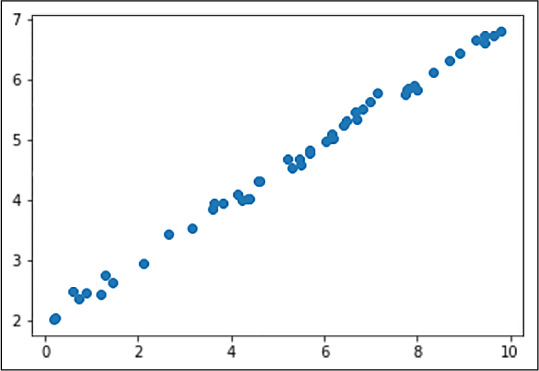
FIGURE 4-1 Synthetic linear dataset
You implement linear regression, so you would try to find an estimation of y, normally written as y_hat, using a straight line: y_hat = w*x + b. The goal of this process would be to find w and b values that make the difference between y and y_hat minimal. For this purpose, you can use the least square error (y – y_hat)2 as your loss function (also called target / cost / objective function), the function you are going to minimize.
In order to find these values using CNTK, you must create a computational graph, that is, define which are the system’s inputs, which parameters you want to be optimized, and what is the order of the operations. With all of this information CNTK, making use of automatic differentiation, optimizes the values of w and b iteration after iteration. After several iterations, the final values of the parameters approach the original values: w_data and b_data. In Figure 4-2 you can find a graphical representation of what the computational network looks like.
)
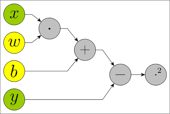
FIGURE 4-2 Computation graph of a linear regression algorithm. The x and y nodes are inputs, w and b nodes are parameters and the remaining nodes are operations. The rightmost node ‘·2’ performs the squaring operation
If you execute operations from left to right, it is called a forward pass. If you run the derivatives of each operation from right to left, it is a called backwards pass. Note that the graph also includes the loss calculation. The outputs of the ‘+’ node are the predictions y_hat and, from then on, the graph is computing the loss. The backward pass optimizes the parameter values (w and b) in such a way as to minimize the loss.
To define your computational graph in CNTK, just use the following lines of code.
x = C.input_variable(1)
y = C.input_variable(1)

w = C.parameter(1)
b = C.parameter(1)

y_hat = x * w + b
loss = C.square(y - y_hat)
Notice that everything here is a placeholder, no computation is done. This code only creates the computational graph. You can see it as a circuit, so you are connecting the different elements but no electricity is flowing. Notice that the ‘*’, ‘-‘ and ‘+’ operators are overloaded by CNTK, so in those cases the operators have a behavior different from the one they have in standard Python. In this case, they create nodes in the computational graph and do not perform any calculations.
Now paint the predictions of the model and the data on a plot. Of course, getting good predictions is not expected, since you are only preparing a visualization function that will be used later. The way in which the visualization is done is by evaluating the model at point x=0 and point x=10 (10 is the value of the scale defined when creating the dataset). After evaluating the model at these points, only one line is drawn between the two values.
def plot():
    plt.scatter(x_data, y_data)  # plot dataset
    x_line = np.array([[0], [scale]], dtype=np.float32)
    y_line = y_hat.eval({x: x_line})
    plt.plot(x_line.flatten(), y_line.flatten())  # plot predictions

plot()
The result of calling the plot function is shown in Figure 4-3. The initial values of w and b are 0, which is why a constant line is painted in 0.
)
FIGURE 4-3 Dataset and initial predictions
Train the model using batch gradient descent (all samples are used in each iteration). You can do that because there is little data. The following script performs 600 iterations and every 50 iterations shows the model loss on the training data (it actually performs 601 iterations in order to show the loss in the last iteration). The learner used is Stochastic Gradient Descent (C.sgd) and uses a learning rate of 0.01.
Note that a test set is not being used and performance is being measured only on the training set. Even if it is not the most correct way to do it, it is a simple experiment that only aims to show how to create and optimize computational networks with CNTK.
learner = C.sgd(y_hat.parameters, lr=0.01)  # learning rate = 0.01
trainer = C.Trainer(y_hat, loss, learner)

for i in range(601):
    trainer.train_minibatch({
        x: x_data,
        y: y_data
    })
    if i % 50 == 0:
        print("{0} - Loss: {1}".format(i, trainer.previous_minibatch_loss_
average))
Figure 4-4 shows the training output and the plot of the predictions. Now the prediction line is no longer zero and is correctly adjusted to the data.
)
FIGURE 4-4 Training log and prediction results
Print the values of w and b and you will obtain some values near the original ones, w ≈ 0.5 and b ≈ 2. Notice that you need to use the property value to access the current value of the parameters:
print("w = {:.3}, b = {:.3}".format(np.asscalar(w.value), np.asscalar(b.value)))
This example is a very simple one, used to explain the key concepts of CNTK. There are a lot of operations (nodes in the computation graph) that can be used in CNTK; indeed there are losses already defined so you do not need to explicitly write the least square error manually (‘-‘ and ‘·2’ nodes), you can use a pre-defined operation that implements that loss. For example, you can replace loss = C.square(y – y_hat) with loss = C.squared_loss(y, y_hat). Defining the least squared error manually is trivial, but for complex ones is not so trivial. You see more examples in the next sections.
Use N-series VMs for GPU acceleration
Although GPUs were initially created to perform computer graphics related tasks, they are now widely used for general-purpose computation (commonly known as general-purpose computing on Graphics Processing Units or GPGPU). This is because the number of cores that a graphics card has is much higher than a typical CPU, allowing parallel operations. Linear algebra is one of the cornerstones of deep learning and the parallelization of operations such as matrix multiplications greatly speeds up training and predictions.
Despite the fact that GPUs are cheaper than other computing hardware (clusters or supercomputers), it is true that buying a GPU can mean a large initial investment and may become outdated after a few years. Azure, the Microsoft cloud, provides solutions to these problems. It enables you to create virtual machines with GPUs, the N-Series virtual machines. Among the N-Series we find two types: the computation-oriented NC-Series and the visualization-oriented NV-Series. Over time, newer versions of graphics cards are appearing and you can make use of them as easily as scaling the machine.
Those machines are great for using the GPU but they need a previous configuration: installing NVIDIA drivers and installing common tools for data science (Python, R, Power BI…).
In this section you create a Deep Learning Virtual Machine (DLVM). This machine comes with pre-installed tools for deep learning. Go to Azure and search for it in the Azure Marketplace (see Figure 4-5).
)
FIGURE 4-5 DLVM in the Azure Marketplace
The procedure is quite similar to creating any other VM. The only difference is when you have to select the size of the machine, which is restricted to NC-Series sizes (see Figure 4-6). For testing purposes select the NC6, which is the cheaper one.
)
FIGURE 4-6 In the second step of the Create Deep Learning Virtual Machine you must select the NC-Series sizes
Once the machine is created you can connect to it by remote desktop and discover that it comes with a lot of tools installed. Figure 4-7 shows a screenshot of the desktop showing some of the pre-installed tools. This allows you to start development quickly without having to worry about installing tools. The Skill 4.2 lists most of the pre-installed applications that a Windows machine has.
)
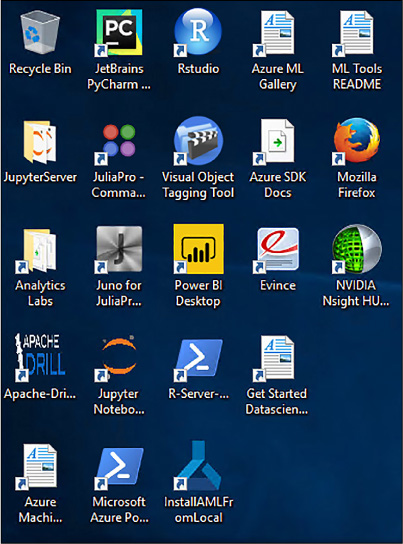
FIGURE 4-7 Desktop of the DLVM with a lot of pre-installed tools
Open a command window and check that the virtual machine has all the NVIDIA drivers installed and detects that the machine has a GPU connected. Use the command nvidia-smi to do this (see Figure 4-8).
)
FIGURE 4-8 Output of the nvidia-smi
Build and train a three-layer feed forward neural network
After building a simple example of computation graph at the beginning of this skill, it is time to build a deep model using the same principles exposed there: create a differentiable computational graph and optimize it by minimizing a cost function. This time you use a famous handwritten digits dataset: MNIST (introduced in LeCun et al., 1998a). The MNIST dataset contains 70000 images of digits from 0 to 9. Images are black and white and have 28x28 pixels. It is common in the machine learning community to use this dataset for tutorials or to test the effectiveness of new models.
The Figure 4-9 shows the implemented architecture: a three-layer feed forward network. This type of networks is characterized by the fact that neurons between contiguous layers are all connected together (dense or fully connected layers). As has been said before, data are black and white 28x28 images, 784 inputs if the images are unrolled in a single-dimensional array. The neural network has two hidden layers of 400 and 200 neurons and an output layer of 10 neurons, one for each class to predict. In order to convert the neural network output into probabilities, softmax is applied to the output of the last layer.
)
FIGURE 4-9 Diagram of the implemented architecture
Each of the neurons in the first layer are connected to all input pixels (784). This means that there is a weight associated with this connection, so in the first layer there are 400 neurons x 784 inputs weights. As in linear regression, each neuron has an intercept term. In machine learning this is also known as bias term. So, the total number of parameters of the first layer are 400 x 784 + 400 bias terms. To obtain the output value of a neuron, what is done internally is to multiply each input by its associated weight, add the results together with the bias and apply the ReLU activation function.
The neurons of the second layer are connected, rather than to the input pixels, to the outputs of the first layer. There are 400 output values from the fist layer and 200 neurons on the second. Each neuron of the second layer is connected to all the neurons of the fist layer (fully connected as before). Following the same calculations as before, the number of parameters of this second layer is 200 x 400 + 200. ReLU is also used as activation function in this layer.
The third and last layer has 10 x 200 + 10 weights. This layer does not use ReLU, but uses softmax to obtain the probability that a given input image is one digit or another. The first neuron in this layer corresponds to the probability of the image being a zero, the second corresponds to the probability of being a one and so on.
The number of neurons and the number of layers are actually hyperparameters of the model. As the number of neurons or layers increases, the expressiveness of the network increases, being able to generate more complex decision boundaries. This is good to some extent, when the number of neurons or layers is very large, in addition to performance problems it is easy to overfit (memorize the training set making the error of generalization very high). More about overfitting has been said in Chapter 2, “Develop machine learning models.”
Create a new Notebook for this exercise. If you are using a Deep Learning Virtual Machine you can run the Jupyter Notebook by clicking the desktop icon (see Figure 4-7).
First write all the necessary imports. Apart from numpy, matplotlib and cntk, you use sklearn to easily load the MNIST dataset.
%matplotlib inline
import matplotlib.pyplot as plt

import cntk as C

import numpy as np

from sklearn.datasets import fetch_mldata
Fetch the data, preprocess it and split it for training and test. The values of each pixel range from 0 to 255 in grayscale. In order to improve the performance of neural networks, always consider normalizing the inputs, which is why each pixel is divided between 255.
# Get the data and save it in your home directory.
mnist = fetch_mldata('MNIST original', data_home='~')
# Rescale the data
X = mnist.data.astype(np.float32) / 255

# One hot encoding
y = np.zeros((70000, 10), dtype=np.float32)
y[np.arange(0, 70000), mnist.target.astype(int)] = 1

# Shuffle samples.
np.random.seed(0)
p = np.random.permutation(len(X))
X, y = X[p], y[p]

# Split train and test.
X_train, X_test = X[:60000], X[60000:]  # 60000 for training
y_train, y_test = y[:60000], y[60000:]  # 10000 for testing
Now that the data is loaded you can create the computational graph.
input_dim = 784
hidden_layers = [400, 200]
num_output_classes = 10

input = C.input_variable((input_dim))
label = C.input_variable((num_output_classes))

def create_model(features):
    with C.layers.default_options(init=C.layers.glorot_uniform(), activation=C.ops.
relu):
        h = features
        for i in hidden_layers:  # for each hidden layer it creates a Dense layer
            h = C.layers.Dense(i)(h)
        return C.layers.Dense(num_output_classes, activation=None)(h)

label_pred = create_model(input)
loss = C.cross_entropy_with_softmax(label_pred, label)
label_error = C.classification_error(label_pred, label)
The variable hidden_layers is a list with the number of hidden neurons of each layer. If you add more numbers to the list, more layers are added to the final neural network. Those layers are initialized using Xavier Glorot uniform initialization (C.layers.glorot_uniform) and are using ReLU (C.ops.relu) as activation function. Xavier’s initialization is a way to set the initial weights of a network with the objective of increasing gradients to speed up training. ReLU activations are commonly used in deep nets because does not suffer from the vanishing gradient problem. The vanishing gradient problem refers to the fact that using sigmoids or hyperbolic tangents (tanh) as activation functions causes the backpropagation signal to degrade as the number of layers increases. This occurs because the derivatives of these functions are between 0 and 1, so consecutive multiplications of small gradients make the gradient of the first layers close to 0. A gradient close to zero means that the weights are practically not updated after each iteration. ReLU activation implements the function max(0, x), so the derivative when x is positive is always 1, avoiding the vanishing gradient problem.
Notice that this time you have used “multi-operation” nodes like the cross entropy and the dense layer. In this way there is no need to manually implement the Softmax function, or implement the matrix multiplication and bias addition that takes place under the wood in a Dense layer. Most of the time, CNTK manages the optimization of these nodes in an even more efficient way than implementing operation by operation.
Once the computational network has been built, all that remains is to feed it with data, execute forward passes, and optimize the value of the parameters with backward passes.
num_minibatches_to_train = 6001
minibatch_size = 64

learner = C.sgd(label_pred.parameters, 0.2)  # constant learning rate -> 0.2
trainer = C.Trainer(label_pred, (loss, label_error), [learner])

# Create a generator
def minibatch_generator(batch_size):
    i = 0
    while True:
        idx = range(i, i + batch_size)
        yield X_train[idx], y_train[idx]
        i = (i + batch_size) % (len(X_train) - batch_size)
# Get an infinite iterator that returns minibatches of size minibatch_size
get_minibatch = minibatch_generator(minibatch_size)


for i in range(0, num_minibatches_to_train):  # for each minibatch
    # Get minibatch using the iterator get_minibatch
    batch_x, batch_y = next(get_minibatch)
    # Train minibatch
    trainer.train_minibatch({
        input: batch_x,
        label: batch_y
    })
    # Show training loss and test accuracy each 500 minibatches
    if i % 500 == 0:
        training_loss = trainer.previous_minibatch_loss_average
        accuracy = 1 - trainer.test_minibatch({
            input: X_test,
            label: y_test
        })
        print("{} - Train Loss: {:.3f}, Test Accuracy: {:.3f}".format(i, training_
loss, accuracy))
Probably the trickiest part of this script is the function minibatch_generator. This function is a Python generator and the variable get_minibatch contains an iterator that returns a different batch each time next(get_minibatch) is called. That part really has nothing to do with CNTK, it’s just a way to get different samples in each batch.
During the training, every 500 minibatches, information is printed on screen about the state of the training: number of minibatches, training loss, and the result of the model evaluation on a test set.
The output of the code fragment above is shown in Figure 4-10.
)
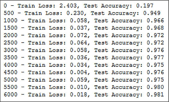
FIGURE 4-10 Training output log, in 6000 minibatches the network reaches 98.1 percent accuracy
It is always convenient to display some examples of the test set and check the performance of the model. The following script creates a grid of plots in which random samples are painted. The title of each plot is the value of its label and the value predicted by the algorithm. If these values do not match, the title will be painted in red to indicate an error.
def plotSample(ax, n):
    ax.imshow(X_test[n].reshape(28,28), cmap="gray_r")
    ax.axis('off')
    # The next two lines use argmax to pass from one-hot encoding to number.
    label = y_test[n].argmax()
    predicted = label_pred.eval({input: [X_test[n]]}).argmax()
    # If correct: black title, if error: red
    title_prop = {"color": "black" if label == predicted else "red"}
    ax.set_title("Label: {}, Predicted: {}".format(label, predicted), title_prop)

np.random.seed(2)  # for reproducibility
fig, ax = plt.subplots(nrows=4, ncols=4, figsize=(10, 6))
for row in ax:
    for col in row:
        plotSample(col, np.random.randint(len(X_test)))
Execute the code. If you use the same random seed, the samples should be like those in Figure 4-11. The value 2 has been chosen as seed because it offers samples in which errors have been made; other random seed values give fewer or no errors. A very interesting way to evaluate neural networks is to look at the errors. In the Figure 4-11 you can see that both misclassifications occur in numbers that are cut below. This kind of visualization can help you to discover bugs in data acquisition or preprocessing. Other common bugs that can be discovered visualizing errors are bad labeled examples, where the algorithm fails because it is actually detecting the correct class but the label is not correct.
)
FIGURE 4-11 Showing examples of predictions, errors are in red
The model is already properly trained and has been proven to work. The example ends here, but consider playing with some hyperparameters like the number of hidden layers/neurons, minibatch size, learning rate, or even other learners different to SGD.
In addition to what you have seen, CNTK offers you many options that have not been discussed: a lot of different operations and losses, data readers, saving trained models to disk, and loading them to later executions.
Determine when to implement a neural network
You have seen something about neural nets on Azure Machine Learning in Skill 2.1. One section of that skill discussed how to create and train neural networks using the Azure Machine Learning module. It was mentioned that, in order to define the structure of the network, it was necessary to write a Net# script. An example was shown on how to construct a neural network with two hidden layers and an output of 10 neurons with Softmax activation. In fact, that example addressed the same problem as in the previous section: classification using the MNIST dataset. If we compare the four Net# lines and the dragging and dropping of Azure Machine Learning modules with the complexity of a CNTK script, you see that there is a big difference. This section lists the advantages and disadvantages of implementing your own neural network in CNTK as opposed to using the Azure Machine Learning module.
With Net# you can:
Create hidden layers and control the number of nodes in each layer.
Specify how layers are to be connected to each other and define special connectivity structures, such as convolutions and weight sharing bundles.
Specify activation functions.
But it has other important limitations such as:
It does not accept regularization (neither L2 nor dropout). This makes the training more difficult, especially with big networks. To avoid this problem, you have to limit the number of training iterations so that the network does not adjust too much to the data (overfitting).
The number of activation functions that you can use are limited and you cannot define your own activation functions either. For example, there is no ReLU activation that are commonly used in deep learning due to their benefits in backpropagation.
There are certain aspects that you cannot modify, such as the batch size of the Stochastic Gradient Descent (SGD). Besides that, you cannot use other optimization algorithms; you can use SGD with momentum, but not others like Adam, or RMSprop.
You cannot define recurrent or recursive neural networks.
Apart from the Net# limitations, the information provided during training in the output log is quite limited and cannot be changed (see Figure 4-12).
)
FIGURE 4-12 Azure Machine Learning output log of a neural network module
With all these shortcomings it is difficult to build a deep neural network that can be successfully trained. But apart from that Net# and log limitations, for deep architectures and to handle a high volume of data (MNIST is actually a small dataset), training a neural network in Azure Machine Learning can be very slow. For all those cases it is preferable to use a GPU-enabled machine. Another drawback of Azure Machine Learning is that it does not allow you to manage the resources dedicated to each experiment. Using an Azure virtual machine you can change the size of the machine whenever you need it.
In CNTK we have all the control during training. For instance, you can stop training when loss goes under a certain threshold. Something as simple as that cannot be done in Azure Machine Learning. All that control comes from the freedom you get from using a programming language.
Programming can become more difficult than managing a graphical interface such as in Azure Machine Learning, but sometimes building a neural network with CNTK is not that much more complicated than writing a complex Net# script. On the other hand, CNTK has a Python API, which is a programming language that is very common in data science and easy to learn. If programming is difficult for you, you should consider using tools like Keras. This tool is a high level deep learning library that uses other libraries like Tensorflow or CNTK for the computational graph implementation. You can implement a digit classifier with far fewer lines than those shown in the example in the previous section and with exactly the same benefits as using CNTK. Also, CNTK is an open source project, so there is a community that offers support for the tool and a lot of examples are available on the Internet.
Deep learning models work very well, especially when working with tons of unstructured data. Those big models are almost impossible to implement in Azure Machine Learning due to the computation limitations, but for simple, small, and structured datasets, the use of Azure Machine Learning can be more convenient and achieve the same results as CNTK.
Figure 4-13 shows a summary table with all the pros and cons listed in this section.
)
FIGURE 4-13 Comparative table showing the pros and cons of implementing a neural network with Azure Machine Learning versus custom implementations with tools like CNTK