Perform calculations on data
- By Curtis Frye and Joan Lambert
- 1/29/2022
Find and correct errors in calculations
Including calculations in a worksheet gives you valuable answers to questions about your data. As is always true, however, it’s possible for errors to creep into your formulas. With Excel, you can find the source of errors in your formulas by identifying the cells used in a specific calculation and describing any errors that have occurred. The process of examining a worksheet for errors is referred to as auditing.
Excel identifies errors in several ways. The first way is to display an error code in the cell that contains the formula generating the error.
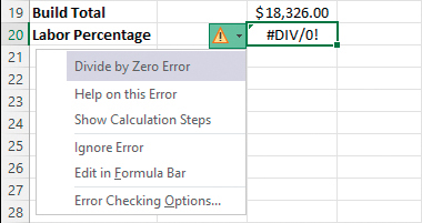
A warning triangle and pound sign indicate an error
When the active cell generates an error, Excel displays an Error button next to it. Pointing to the button displays information about the error, and selecting the button displays a menu of options for handling the error.
The following table explains the most common error codes.
Error code |
Description |
|---|---|
##### |
The column isn’t wide enough to display the value. |
#VALUE! |
The formula has the wrong type of argument, such as text in a cell where a numerical value is required. |
#NAME? |
The formula contains text that Excel doesn’t recognize, such as an unknown named range. |
#REF! |
The formula refers to a cell that doesn’t exist, which can happen whenever cells are deleted. |
#DIV/0! |
The formula attempts to divide by zero. |
Another technique you can use to find the source of formula errors is to ensure that the appropriate cells are providing values for the formula. You can identify the source of an error by having Excel trace a cell’s precedents, which are the cells with values used in the active cell’s formula. You can also audit your worksheet by identifying cells with formulas that use a value from a particular cell. Cells that use another cell’s value in their calculations are known as dependents, meaning that they depend on the value in the other cell to derive their own value. They are identified in Excel by tracer arrows. If the cells identified by the tracer arrows aren’t the correct cells, you can hide the arrows and correct the formula.
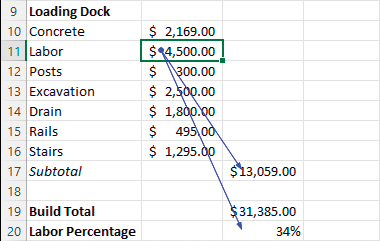
Tracing a cell’s dependents
If you prefer to have the elements of a formula error presented as text in a dialog, you can use the Error Checking tool to locate errors one after the other. You can choose to ignore the selected error or move to the next or the previous error.
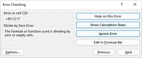
Identify and manage errors from the Error Checking window
 TIP
TIP
You can have the Error Checking tool ignore formulas that don’t use every cell in a region (such as a row or column). To do so, on the Formulas tab of the Excel Options dialog, clear the Formulas Which Omit Cells In A Region checkbox. Excel will no longer mark these cells as an error.
When you just want to display the results of each step of a formula and don’t need the full power of the Error Checking tool, you can use the Evaluate Formula dialog to move through each element of the formula. The Evaluate Formula dialog is particularly useful for examining formulas that don’t produce an error but aren’t generating the result you expect.
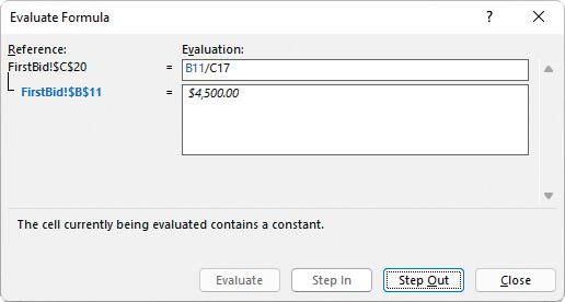
Step through formulas in the Evaluate Formula window
Finally, you can monitor the value in a cell regardless of where you are in your workbook by opening a Watch Window that displays the value in the cell. For example, if one of your formulas uses values from cells in other worksheets or even other workbooks, you can set a watch on the cell that contains the formula, and then change the values in the other cells. As you change the precedent values, the formula result changes in the Watch Window. When you’re done watching the formula, you can delete the watch and close the Watch Window.
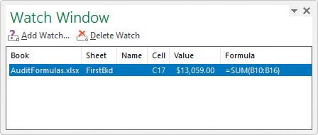
Monitor formula results in the Watch Window
To display information about a formula error
Select the cell that contains the error.
Point to the error indicator next to the cell to display information about the error.
Select the error indicator to display options for correcting or learning more about the error.
To identify the cells that a formula references
Select the cell that contains the formula.
On the Formulas tab, in the Formula Auditing group, select Trace Precedents.
To identify formulas that reference a specific cell
Select the cell.
In the Formula Auditing group, select Trace Dependents.
To remove tracer arrows
In the Formula Auditing group, do one of the following:
To remove all the arrows, select the Remove Arrows button (not its arrow).
To remove only precedent or dependent arrows, select the Remove Arrows arrow, and then select Remove Precedent Arrows or Remove Dependent Arrows.
To evaluate a formula one calculation at a time
Select the cell that contains the formula you want to evaluate.
In the Formula Auditing group, select Evaluate Formula.
In the Evaluate Formula dialog, select Evaluate. Excel replaces the underlined calculation with its result.
Do either of the following:
Select Step In to move forward by one calculation.
Select Step Out to move backward by one calculation.
When you finish, select Close.
To change error display options
Display the Formulas page of the Excel Options dialog.
In the Error Checking section, select or clear the Enable background error checking checkbox.
Select the Indicate errors using this color button and select a color.
Select Reset Ignored Errors to return Excel to its default error indicators.
In the Error checking rules section, select or clear the checkboxes next to errors you want to indicate or ignore, respectively.
To watch the values in a cell range
Select the cell range you want to watch.
In the Formula Auditing group, select the Watch Window button.
In the Watch Window dialog, select Add Watch.
In the Add Watch dialog, confirm the cell range, and then select Add.
To delete a watch
Select the Watch Window button.
In the Watch Window dialog, select the watch you want to delete.
Select Delete Watch.