Perform calculations on data

Summarize data that meets specific conditions

Another use for formulas is to display messages when certain conditions are met. This kind of formula is called a conditional formula. One way to create a conditional formula in Excel is to use the IF function. Selecting the Insert Function button next to the formula bar and then choosing the IF function displays the Function Arguments dialog with the fields required to create an IF formula.

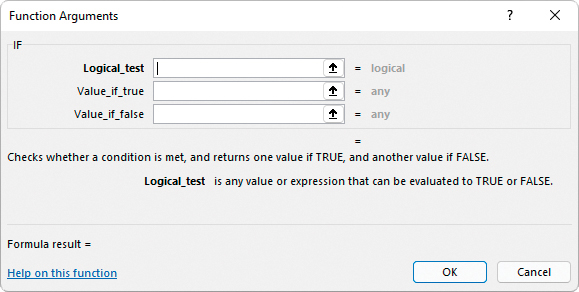
The Function Arguments dialog for an IF formula

When you work with an IF function, the Function Arguments dialog displays three input boxes:

• Logical_test The condition you want to check.

• Value_if_true The value to display if the condition is met. This could be a cell reference, or a number or text enclosed in quotes.

• Value_if_false The value to display if the condition is not met.

The following table displays other conditional functions you can use to summarize data.

To create a formula that uses the AVERAGEIF function, you define the range to be examined for the criterion, the criterion, and, if required, the range from which to draw the values. As an example, consider a worksheet that lists each customer’s ID number, name, state, and total monthly shipping bill. If you want to find the average order of customers from the state of Washington (abbreviated in the worksheet as WA), you can create the formula =AVERAGEIF(C3:C6, “WA”, D3:D6).

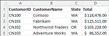
Sample data that illustrates the preceding example

The AVERAGEIFS, SUMIFS, and COUNTIFS functions extend the capabilities of the AVERAGEIF, SUMIF, and COUNTIF functions to allow for multiple criteria. For example, if you want to find the sum of all orders of at least $100,000 placed by companies in Washington, you can create the formula =SUMIFS(D2:D5, C2:C5, “=WA”, D2:D5, “>=100000”).

The AVERAGEIFS and SUMIFS functions start with a data range that contains values that the formula summarizes. You then list the data ranges and the criteria to apply to that range. In generic terms, the syntax is =AVERAGEIFS(data_range, criteria_range1, criteria1[,criteria_range2, criteria2...]). The part of the syntax in brackets (which aren’t used when you create the formula) is optional, so an AVERAGEIFS or SUMIFS formula that contains a single criterion will work. The COUNTIFS function, which doesn’t perform any calculations, doesn’t need a data range; you just provide the criteria ranges and criteria. For example, you could find the number of customers from Washington who were billed at least $100,000 by using the formula =COUNTIFS(C2:C5, “=WA”, D2:D5, “>=100000”).

You can use the IFERROR function to display a custom error message instead of relying on the default Excel error messages to explain what happened. For example, you could create this type of formula to employ the VLOOKUP function to look up a customer’s name in the second column of a table named Customers based on the customer identification number entered into cell G8. That formula might look like this: =IFERROR(VLOOKUP(G8,Customers,2,FALSE),”Customer not found”). If the function finds a match for the customer ID in cell G8, it displays the customer’s name; if not, it displays the text “Customer not found.”

To summarize data by using the IF function

• Use the syntax =IF(logical_test, value_if_true, value_if_false) where:

  • logical_test is the logical test to be performed.

  • value_if_true is the value the formula returns if the test is true.

  • value_if_false is the value the formula returns if the test is false.

To count cells that contain numbers in a range

• Use the syntax =COUNT(range), where range is the cell range in which you want to count cells.

To count cells that are non-blank

• Use the syntax =COUNTA(range), where range is the cell range in which you want to count cells.

To count cells that contain a blank value

• Use the syntax =COUNTBLANK(range), where range is the cell range in which you want to count cells.

To count cells that meet one condition

• Use the syntax =COUNTIF(range, criteria) where:

  • range is the cell range that might contain the criteria value.

  • criteria is the logical test used to determine whether to count the cell.

To count cells that meet multiple conditions

• Use the syntax =COUNTIFS(criteria_range1, criteria1, criteria_range2, criteria2,…) where for each criteria_range and criteria pair:

  • criteria_range is the cell range that might contain the criteria value.

  • criteria is the logical test used to determine whether to count the cell.

To find the sum of data that meets one condition

• Use the syntax =SUMIF(range, criteria, sum_range) where:

  • range is the cell range that might contain the criteria value.

  • criteria is the logical test used to determine whether to include the cell.

  • sum_range is the range that contains the values to be included if the range cell in the same row meets the criterion.

To find the sum of data that meets multiple conditions

• Use the syntax =SUMIFS(sum_range, criteria_range1, criteria1, criteria_range2, criteria2,…) where:

  • sum_range is the range that contains the values to be included if all criteria_range cells in the same row meet all criteria.

  • criteria_range is the cell range that might contain the criteria value.

  • criteria is the logical test used to determine whether to include the cell.

To find the average of data that meets one condition

• Use the syntax =AVERAGEIF(range, criteria, average_range) where:

  • range is the cell range that might contain the criteria value.

  • criteria is the logical test used to determine whether to include the cell.

  • average_range is the range that contains the values to be included if the range cell in the same row meets the criterion.

To find the average of data that meets multiple conditions

• Use the syntax =AVERAGEIFS(average_range, criteria_range1, criteria1, criteria_range2, criteria2,…) where:

  • average_range is the range that contains the values to be included if all criteria_range cells in the same row meet all criteria.

  • criteria_range is the cell range that might contain the criteria value.

  • criteria is the logical test used to determine whether to include the cell.

To display a custom message if a cell contains an error

• Use the syntax =IFERROR(value, value_if_error) where:

  • value is a cell reference or formula.

  • value_if_error is the value to be displayed if the value argument returns an error.