Customizing a pivot table
- By Bill Jelen
- 1/10/2022
Making report layout changes
Excel offers three report layout styles. The Excel team continues to offer the Compact layout as the default report layout. If you prefer a different layout, change it using the default settings for pivot tables.
If you consider three report layouts, and the ability to show subtotals at the top or bottom, plus choices for blank rows and Repeat All Item Labels, you have 16 different layout possibilities available.
Layout changes are controlled in the Layout group of the Design tab, as shown in Figure 3-8. This group offers four icons:
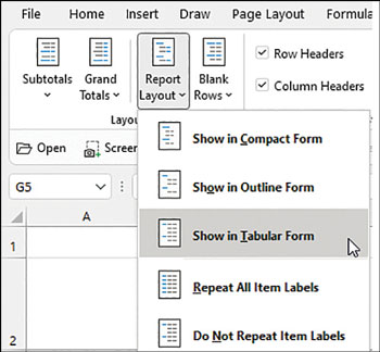
FIGURE 3-8 The Layout group on the Design tab offers different layouts and options for totals.
Subtotals—Moves subtotals to the top or bottom of each group or turns them off.
Grand Totals—Turns the grand totals on or off for rows and columns.
Report Layout—Uses the Compact, Outline, or Tabular forms. Offers an option to repeat item labels.
Blank Rows—Inserts or removes blank lines after each group.
 Note
Note
You mathematicians in the audience might think that 3 layouts × 2 repeat options × 2 subtotal location options × 2 blank row options would be 24 layouts. However, choosing Repeat All Item Labels does not work with the Compact layout, thus eliminating 4 of the combinations. In addition, Subtotals At The Top Of Each Group does not work with the Tabular layout, eliminating another 4 combinations.
Using the Compact layout
By default, all new pivot tables use the Compact layout that you saw in Figure 3-6. In this layout, multiple fields in the row area are stacked in column A. Note in the figure that the Consultants sector and the Andrew Spain Consulting customer are both in column A.
The Compact form is suited for using the Expand and Collapse icons. If you select one of the Sector value cells such as Associations in A5 and then click the Collapse Field icon on the Analyze tab, Excel hides all the customer details and shows only the sectors, as shown in Figure 3-9.
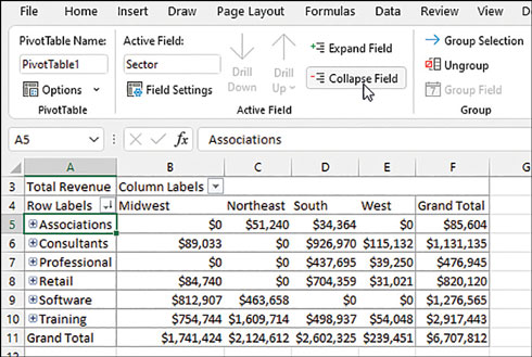
FIGURE 3-9 Click the Collapse Field icon to hide levels of detail.
After a field is collapsed, you can show detail for individual items by using the plus icons in column A, or you can click Expand Field on the PivotTable Analyze tab to see the detail again.
 Tip
Tip
If you select a cell in the innermost row field and click Expand Field on the Options tab, Excel displays the Show Detail dialog box, as shown in Figure 3-10, to enable you to add a new innermost row field.
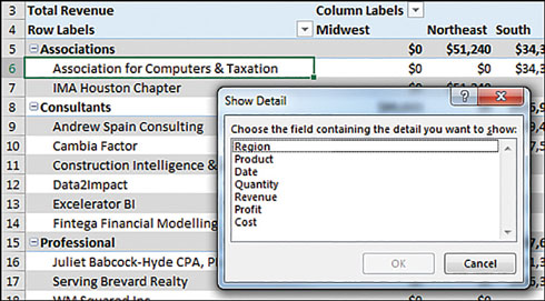
FIGURE 3-10 When you attempt to expand the innermost field, Excel offers to add a new innermost field.
Using the Outline layout
When you select Design, Layout, Report Layout, Show In Outline Form, Excel puts each row field in a separate column. The pivot table shown in Figure 3-11 is one column wider, with revenue values starting in C instead of B. This is a small price to pay for allowing each field to occupy its own column. Soon, you will find out how to convert a pivot table to values so you can further sort or filter. When you do this, you will want each field in its own column.
The Excel team added the Repeat All Item Labels option to the Report Layout tab starting in Excel 2010. This alleviated a lot of busy work because it takes just two clicks to fill in all the blank cells along the outer row fields. Choosing to repeat the item labels causes values to appear in cells A6:A7, A9:A14, as shown in Figure 3-11.
Figure 3-11 shows the same pivot table from before, now in Outline form and with labels repeated.
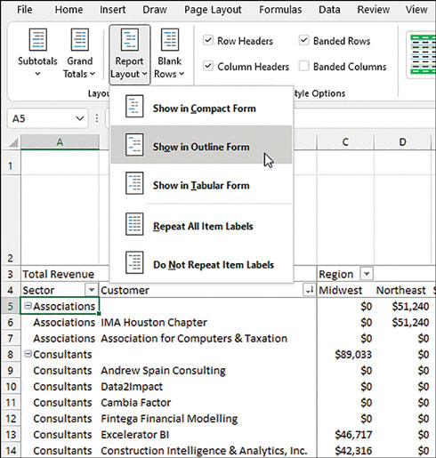
FIGURE 3-11 The Outline layout puts each row field in a separate column.
 Caution
This layout is suitable if you plan to copy the values from the pivot table to a new location for further analysis. Although the Compact layout offers a clever approach by squeezing multiple fields into one column, it is not ideal for reusing the data later.
By default, both the Compact and Outline layouts put the subtotals at the top of each group. You can use the Subtotals drop-down menu on the Design tab to move the totals to the bottom of each group, as shown in Figure 3-12. In Outline view, this causes a not-really-useful heading row to appear at the top of each group. Cell A5 contains “Associations” without any additional data in the columns to the right. Consequently, the pivot table occupies 44 rows instead of 37 rows because each of the 7 sector categories has an extra header.
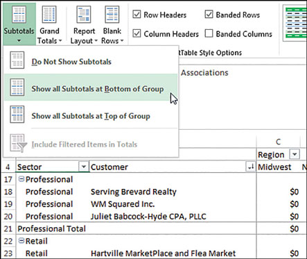
FIGURE 3-12 With subtotals at the bottom of each group, the pivot table occupies several more rows.
Using the traditional Tabular layout
Figure 3-13 shows the Tabular layout. This layout is similar to the one that has been used in pivot tables since their invention through Excel 2003. In this layout, the subtotals can never appear at the top of the group. The Repeat All Item Labels works with this layout, as shown in Figure 3-13.
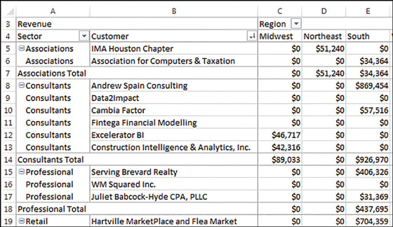
FIGURE 3-13 The Tabular layout is similar to pivot tables in legacy versions of Excel.
The Tabular layout is the best layout if you expect to use the resulting summary data in a subsequent analysis. If you wanted to reuse the table in Figure 3-13, you would do additional “flattening” of the pivot table by choosing Subtotals, Do Not Show Subtotals and Grand Totals, Off For Rows And Columns.
Case study: Converting a pivot table to values
Say that you want to convert the pivot table shown in Figure 3-13 to be a regular data set that you can sort, filter, chart, or export to another system. You don’t need the Sectors totals in rows 7, 14, 18, and so on. You don’t need the Grand Total at the bottom. And, depending on your future needs, you might want to move the Region field from the Columns area to the Rows area. This would allow you to add Cost and Profit as new columns in the final report.
Finally, you want to convert from a live pivot table to static values. To make these changes, follow these steps
Select any cell in the pivot table.
From the Design tab, select Grand Totals, Off For Rows And Columns.
Select Design, Subtotals, Do Not Show Subtotals.
Drag the Region tile from the Columns area in the PivotTable Fields list. Drop this field between Sector and Customer in the Rows area.
Check Profit and Cost in the top of the PivotTable Fields list. Because both fields are numeric, they move to the Values area and appear in the pivot table as new columns. Rename both fields using the Current Field box on the PivotTable Analyze tab. The report is now a contiguous solid block of data, as shown in Figure 3-14.
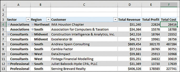
FIGURE 3-14 The pivot table now contains a solid block of data.
Select one cell in the pivot table. Press Ctrl+* to select all the data in the pivot table.
Press Ctrl+C to copy the data from the pivot table.
Select a blank section of a worksheet.
Right-click. To the right of the words “Paste Special” is a greater-than sign that leads to a flyout with 14 ways to Paste Special Choose Paste Values And Number Formatting, as shown in Figure 3-15. Excel pastes a static copy of the report to the worksheet.
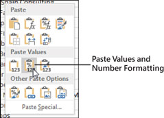
FIGURE 3-15 Use Paste Values And Number Formatting to create a static version of the data.
If you no longer need the original pivot table, select the entire pivot table and press the Delete key to clear the cells from the pivot table and free up the area of memory that was holding the pivot table cache. One way to select the entire pivot table is to use the Select drop-down menu on the PivotTable Analyze tab and choose Entire PivotTable.
The result is a solid block of summary data. These 27 rows are a summary of the 500+ rows in the original data set, but they also are suitable for exporting to other systems.
)
)
)
)
)
)
)
)
)
Controlling blank lines, grand totals, and other settings
Additional settings on the Design tab enable you to toggle various elements.
The Blank Rows drop-down menu offers the choice Insert Blank Line After Each Item. This setting applies only to pivot tables with two or more row fields. Blank rows are not added after each item in the inner row field. You see a blank row after each group of items in the outer row fields. As shown in Figure 3-16, the blank row after each sector makes the report easier to read. However, if you remove Sector from the report, you have only Customer in the row fields, and no blank rows appear (see Figure 3-17).
)
)
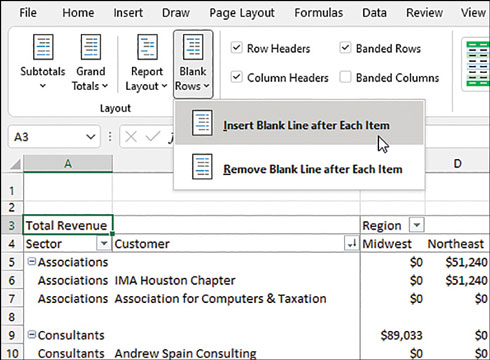
FIGURE 3-16 The Blank Rows setting makes the report easier to read.
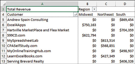
FIGURE 3-17 Blank rows will not appear when there is only one item in the row field.
Grand totals can appear at the bottom of each column and/or at the end of each row, or they can be turned off altogether. Settings for grand totals appear in the Grand Totals drop-down menu of the Layout group on the Design tab. The wording in this drop-down menu is a bit confusing, so Figure 3-18 shows what each option provides. The default is to show grand totals for rows and columns.
)
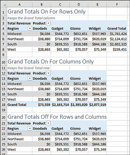
FIGURE 3-18 The wording is confusing, but you can toggle off the grand total column, row, or both.
If you want a grand total column but no grand total at the bottom, choose On For Rows Only, as shown at the top of Figure 3-18. To me, this seems backward. To keep the grand total column, you have to choose to turn on grand totals for rows only. I guess the rationale is that each cell in F5:F8 is a grand total of the row to the left of the cell. Hence, you are showing the grand totals for all the rows but not for the columns. Perhaps someday Microsoft will ship a version of Excel in English-Midwest where this setting would be called “Keep the Grand Total Column.” But for now, it remains confusing.
In a similar fashion, to show a grand total row but no grand total column, you open the Grand Totals menu and choose On For Columns Only. Again, in some twisted version of the English language, cell B18 is totaling the cells in the column above it.
The final choice, Off For Rows And Columns, is simple enough. Excel shows neither a grand total column nor a grand total row.
Tip
You can abandon these confusing menu choices by using the right-click menu. If you right-click on any cell that has the words “Grand Total,” you can choose Remove Grand Total.
Back in Excel 2003, pivot tables were shown in Tabular layout and logical headings such as Region and Product would appear in the pivot table, as shown in the top pivot table in Figure 3-19. When the Excel team switched to Compact form, they replaced those headings with Row Labels and Column Labels. These add nothing to the report. To toggle off those headings, look on the far-right side of the PivotTable Analyze tab for an icon called Field Headers and click it to remove Row Labels and Column Labels from your pivot tables in Compact form.
)
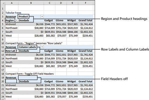
FIGURE 3-19 The Compact form replaces useful headings with Row Labels. You can turn these off.
Caution
When you arrange several pivot tables vertically, as in Figure 3-19, you’ll notice that changes in one pivot table change the column widths for the entire column, often causing #### to appear in the other pivot tables. By default, Excel changes the column width to AutoFit the pivot table but ignores anything else in the column. To turn off this default behavior, right-click each pivot table and choose PivotTable Options. In the first tab of the Options dialog box, the second-to-last check box is AutoFit Column Widths On Update. Clear this check box. This is another setting that you might want to adjust in Pivot Table Defaults. See Tip 5 in Chapter 14.