Describe fundamental principles of machine learning on Azure
- By Julian Sharp
- 2/1/2022
- Skill 2.1: Identify common machine learning types
- Skill 2.2: Describe core machine learning concepts
- Skill 2.3: Identify core tasks in creating a machine learning solution
Skill 2.2: Describe core machine learning concepts
Machine learning has several common concepts that apply when building machine learning models. These concepts apply no matter which tools, languages, or frameworks that you use. This section explains the fundamental concepts and processes involved in building machine learning models.
Understand the machine learning workflow
Building a machine learning model follows the process outlined in Figure 2-7. It is important to note that building a model is an iterative process where the model is evaluated and refined.
)
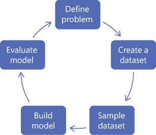
FIGURE 2-7 Machine learning workflow
First, you define the problem. This means translating the business problem into a machine learning problem statement. For example, if you are asked to understand how groups of customers behave, you would transform that as create a clustering model using customer data.
In the example used in this chapter, we want to discover how much activity a student needs to undertake to pass the exam. So far, we have kept this simple just by looking at the hours studied, but we have been asked to look at other factors such as whether they have completed the labs and their choice of degree subject. We could transform these into the following problem statements:
Create a regression model to predict a student’s score for the exam using their degree subject and their exam preparation activities.
Create a classification model to predict if a student will pass the exam using their degree subject and their exam preparation activities.
Identify the features and labels in a dataset for machine learning
The next step in the machine learning workflow is to create a dataset. Data is the most important asset you have as you use data to train your model. If your data is incomplete or inaccurate, then it will have a major impact on how well your model performs.
You must first collect your data. This can mean extracting data from multiple systems, transforming, cleansing, and importing the data.
 Exam Tip
How to extract and transform data is outside the scope of this exam.
We will start with the same dataset we used earlier in this chapter with some additional exam results, as shown in the table in Figure 2-8.
)
FIGURE 2-8 Dataset
Identify labels
If you are using supervised training—for example, a regression or a classification model—then you need to select the label(s) from your dataset. Labels are the columns in the dataset that the model predicts.
For a regression model, the Score column is the label you would choose, as this is a numeric value. Regression models are used to predict a range of values.
For a classification model, the Pass column is the label you would choose as this column has distinct values. Classification models are used to predict from a list of distinct categories.
Feature selection
A feature is a column in your dataset. You use features to train the model to predict the outcome. Features are used to train the model to fit the label. After training the model, you can supply new data containing the same features, and the model will predict the value for the column you have selected as the label.
The possible features in our dataset are the following:
Background
Hours Studied
Completed Labs
In the real world, you will have other possible features to choose from.
Feature selection is the process of selecting a subset of relevant features to use when building and training the model. Feature selection restricts the data to the most valuable inputs, reducing noise and improving training performance.
Feature engineering
Feature engineering is the process of creating new features from raw data to increase the predictive power of the machine learning model. Engineered features capture additional information that is not available in the original feature set.
Examples of feature engineering are as follows:
Aggregating data
Calculating a moving average
Calculating the difference over time
Converting text into a numeric value
Grouping data
Models train better with numeric data rather than text strings. In some circumstances, data that visually appears to be numeric may be held as text strings, and you need to parse and convert the data type into a numeric value.
In our dataset, the background column, the degree subject names for our students, may not perform well when we evaluate our model. One option might be to classify the degree subjects into humanities and sciences and then to convert to a Boolean value, such as IsScienceSubject, with values of 1 for True and 0 for False.
Bias
Bias in machine learning is the impact of erroneous assumptions that our model makes about our data. Machine learning models depend on the quality, objectivity, and quantity of data used to train it. Faulty, incomplete, or prejudicial data can result in a poorly performing model.
In Chapter 1, we introduced the Fairness principle and how an AI model should be concerned with how data influences the model’s prediction to help eliminate bias. You should therefore be conscious of the provenance of the data you are using in your model. You should evaluate the bias that might be introduced by the data you have selected.
A common issue is that the algorithm is unable to learn the true signal from the data, and instead, noise in the data can overly influence the model. An example from computer vision is where the army attempted to build a model that was able to find enemy tanks in photographs of landscapes. The model was built with many different photographs with and without tanks in them. The model performed well in testing and evaluation, but when deployed, the model was unable to find tanks. Eventually, it was realized that all pictures of tanks were taken on cloudy days, and all pictures without tanks were taken on sunny days. They had built a model that identifies whether a photograph was of a sunny or a cloudy day; the noise of the sunlight biased the model. The problem of bias was resolved by adding additional photographs into the dataset with varying degrees of cloud cover.
It can be tempting to select all columns as features for your model. You may then find when you evaluate the model that one column significantly biases the model, with the model effectively ignoring the other columns. You should consider removing that column as a feature if it is irrelevant.
Normalization
A common cause of bias in a model is caused by data in numeric features having different ranges of values. Machine learning algorithms tend to be influenced by the size of values, so if one feature ranges in values between 1 and 10 and another feature between 1 and 100, the latter column will bias the model toward that feature.
You mitigate possible bias by normalizing the numeric features, so they are on the same numeric scale.
After feature selection, feature engineering, and normalization, our dataset might appear as in the table in Figure 2-9.
)
FIGURE 2-9 Normalized dataset
Describe how training and validation datasets are used in machine learning
After you have created your dataset, you need to create sample datasets for use in training and evaluating your model.
Typically, you split your dataset into two datasets when building a machine learning model:
Training The training dataset is the sample of data used to train the model. It is the largest sample of data used when creating a machine learning model.
Testing The testing, or validation, dataset is a second sample of data used to provide a validation of the model to see if the model can correctly predict, or classify, using data not seen before.
A common ratio between training and validation data volumes is 70:30, but you may vary this ratio depending on your needs and size of your data.
You need to be careful when splitting the data. If you simply take the first set of rows, then you may bias your data by date created or however the data is sorted. You should randomize the selected data so that both training and testing datasets are representative of the entire dataset.
For example, we might split our dataset as shown in Figure 2-10.
)
FIGURE 2-10 Training and testing datasets
Describe how machine learning algorithms are used for model training
A machine learning model learns the relationships between the features and the label in the training dataset.
It is at this point that you select the algorithm to train the model with.
The algorithm finds patterns and relationships in the training data that map the input data features to the label that you want to predict. The algorithm outputs a machine learning model that captures these patterns.
Training a model can take a significant amount of time and processing power. The cloud has enabled data scientists to use the scalability of the cloud to build models more quickly and with more data than can be achieved with on-premises hardware.
After training, you use the model to predict the label based on its features. You provide the model with new input containing the features (Hours Studied, Completed Labs) and the model will return the predicted label (Score or Pass) for that student.
Select and interpret model evaluation metrics
After a model has been trained, you need to evaluate how well the model has performed. First, you score the model using the data in the testing dataset that was split earlier from the dataset. This data has not been seen by the model, as it was not used to build the model.
To evaluate the model, you compare the prediction values for the label with the known actual values to obtain a measure of the amount of error. You then create metrics to help gauge the performance of the model and explore the results.
There are different ways to measure and evaluate regression, classification, and clustering models.
Evaluate regression models
When evaluating a regression model, you estimate the amount of error in the predicted values.
To determine the amount of error in a regression model, you measure the difference between the actual values you have for the label and the predicted values for the label. These are known as the residual values. A way to represent the amount of error is to draw a line from each data point perpendicular to the best fit line, as shown in Figure 2-11.
)
FIGURE 2-11 Regression errors
The length of the lines indicates the size of residual values in the model. A model is considered to fit the data well if the difference between actual and predicted values is small.
The following metrics can be used when evaluating regression models:
Mean absolute error (MAE) Measures how close the predictions are to the actual values; lower is better.
Root mean squared error (RMSE) The square root of the average squared distance between the actual and the predicted values; lower is better.
Relative absolute error (RAE) Relative absolute difference between expected and actual values; lower is better.
Relative squared error (RSE) The total squared error of the predicted values by dividing by the total squared error of the actual values; lower is better.
Mean Zero One Error (MZOE) If the prediction was correct or not with values 0 or 1.
Coefficient of determination (R2 or R-squared) A measure of the variance from the mean in its predictions; the closer to 1, the better the model is performing.
We will see later that Azure Machine Learning calculates these metrics for us.
Evaluate classification models
In a classification model with distinct categories predicted, we are interested where the model gets it right or gets it wrong.
A common way to represent how a classification model is right or wrong is to create a confusion matrix. In a confusion matrix, the numbers of true positives, true negatives, false positives, and false negatives are shown:
True Positive The model predicted true, and the actual is true.
True Negative The model predicted false, and the actual is false.
False Positive The model predicted true, and the actual is false.
False Negative The model predicted negative, and the actual is true.
The total number of true positives is shown in the top-left corner, and the total number of true negatives is shown in the bottom-right corner. The total number of false positives is shown in the top-right corner, and the total number of false negatives is shown in the bottom-left corner, as shown in Figure 2-12.
)
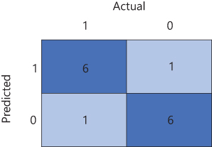
FIGURE 2-12 Confusion matrix
From the values in the confusion matrix, you can calculate metrics to measure the performance of the model:
Accuracy The number of true positives and true negatives; the total of correct predictions, divided by the total number of predictions.
Precision The number of true positives divided by the sum of the number of true positives and false positives.
Recall The number of true positives divided by the sum of the number of true positives and false negatives.
F-score Combines precision and recall as a weighted mean value.
Area Under Curve (AUC) A measure of true positive rate over true negative rate.
All these metrics are scored between 0 and 1, with closer to 1 being better.
We will see later that Azure Machine Learning generates the confusion matric and calculates these metrics for us.
Evaluate clustering models
Clustering models are created by minimizing the distance of a data point to the center point of its cluster.
The Average Distance to Cluster Center metric is used when evaluating clustering models and is a measure of how focused the clusters are. The lower the value, the better.