Basic Data Preparation Challenges

Extracting Information from Text Columns

In the preceding exercises, you extracted meaningful information from delimiter-separated codes by using the Split Column by Delimiter transformation. In the next exercise, you will tackle a common challenge: how to extract meaningful data from unstructured textual data. While this challenge can be simple if your data is relatively consistent, you need a wider arsenal of techniques to address inconsistent data.

Exercise 2-4: Extracting Hyperlinks from Messages

In this exercise you will work on a workbook that contains imported Facebook posts from the official Microsoft Press Facebook page. Specifically, you will extract the hyperlinks from posts that were shared by Microsoft Press. While some hyperlinks are easily extracted, as they start with the prefix “http://”, there are plenty of edge cases that cannot be easily addressed.

Before you start, download the workbook C02E04.xlsx from https://aka.ms/DataPwrBIPivot/downloads and save it in C:\Data\C02.

1. Start a new blank Excel workbook or a new Power BI Desktop report.

2. Follow these steps to import C02E04.xlsx to the Power Query Editor:

   1. In Excel: On the Data tab, select Get Data, From File, From Workbook.

      In Power BI Desktop: In the Get Data drop-down menu, select Excel.

   2. Select the file C02E04.xlsx and select Import.

   3. In the Navigator dialog box that opens, select Sheet1 and then click Edit.

   The Power Query Editor opens, and you see that the Message column contains free text. Before you extract the hyperlinks from the Message column, to achieve your goal, as illustrated in Figure 2-8, you first need to duplicate the column to keep the original message intact, so select the Message column, and from the Add Column tab, select Duplicate Column.

   

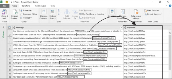
   FIGURE 2-8 You can extract hyperlinks from Microsoft Press Facebook posts.

3. Rename the new column Hyperlink.

4. To extract the hyperlink from the new column, you can use the hyperlink prefix “http://” as a delimiter and split the column, so select the Hyperlink column, and on the Transform tab, select Split Column and then select By Delimiter.

5. In the Split Column by Delimiter dialog box that opens, do the following:

   1. Enter “http://” in the text box below Custom.

   2. Select the Left-Most Delimiter option at Split At radio buttons and click OK to close the dialog box.

   You can now see that the Hyperlink column has been split into two columns: Hyperlink.1 and Hyperlink.2. But how can you extract hyperlinks that start with “https://” or perhaps just “www.”?

6. In Applied Steps, select the step Split Column by Delimiter.

7. Ensure that your formula bar in the Power Query Editor is active. If you don’t see it, go to the View tab and select the Formula Bar check box. Now, you can see the following formula, which was generated in step 7:

   = Table.SplitColumn(#"Renamed Columns", "Hyperlink",
   Splitter.SplitTextByEachDelimiter({"http://"},
   QuoteStyle.Csv, false), {"Hyperlink.1", "Hyperlink.2"})

8. To split the Hyperlink column by additional delimiters, you can change the function name from Splitter.SplitTextByEachDelimiter to Splitter.SplitTextByAnyDelimiter. Now, you can add the new delimiters “https://” and “www.”. You can see in the formula above that “https://” is wrapped in double quotes inside curly brackets. Curly brackets represent lists in the M language of Power Query. You can now add multiple items to the list by adding double-quoted comma-separated delimiters, like this: {“http://”, “https://”, “www.”}.

   Here is the complete modified formula:

   = Table.SplitColumn(#"Renamed Columns", "Hyperlink",
   Splitter.SplitTextByAnyDelimiter({"http://", "https://", "www."},
   QuoteStyle.Csv, false), {"Hyperlink.1", "Hyperlink.2"})

9. Thanks to the addition of “www.” as a delimiter, you can now see in the Preview pane that in line 8 a new hyperlink was detected in the Hyperlink.2 column: microsoftpressstore.com/deals.

10. Go back to the last step in Applied Steps.

11. To audit the results in Hyperlink.2, in row 15, notice that the original message contains additional text following the hyperlink. To remove the trailing text from the hyperlink, you can assume that the hyperlinks end with a space character and split Hyperlink.2. To do it, select the Hyperlink.2 column. On the Transform tab, select Split Column and then select By Delimiter. The Split Column by Delimiter dialog box opens.

    1. Select Space from the Select or Enter Delimiter drop-down.

    2. Select the Left-Most Delimiter option for Split At radio buttons and click OK to close the dialog box.

12. Remove the Hyperlink.2.2 column.

    To continue auditing the results in Hyperlink.2, scroll down until you find the first null value, in row 29. A null value means that you couldn’t detect any hyperlink in the message. But if you take a closer look at the message in the Hyperlink.1 column, you can see that it contains the bolded hyperlink, as shown in the line Discover Windows containers in this free ebook. Download here: aka.ms/containersebook.

    The next challenge is to extract the hyperlinks whose domain name is aka.ms and include them in the Hyperlink column. This challenge is rather complex because after you split the Message column by the delimiter aka.ms, the domain name will be removed from the split results. When you applied “www.” in step 8, “www.” was removed from the hyperlink, but that was a safe manipulation. You were taking the risk that the resulted hyperlink will work well without the “www.” prefix because it is common to omit this prefix from hyperlinks (e.g., www.microsoft.com and microsoft.com lead to the same website).

    You need to find a way to split by aka.ms, and you must find a way to return the domain name, but only for rows that contain that domain. You will soon learn how to do it by using a conditional column. But first, you need to add aka.ms to the list of delimiters.

13. In Applied Steps, select again the first Split Column by Delimiter step, which you modified in step 8, and add aka.ms to the list of delimiters. Here is the modified formula:

    = Table.SplitColumn(#"Renamed Columns", "Hyperlink",
    Splitter.SplitTextByAnyDelimiter({"http://", "https://", "www.", "aka.ms"},
    QuoteStyle.Csv, false), {"Hyperlink.1", "Hyperlink.2"})

    You can now see in row 29 that the hyperlink is /containersebook. In the next steps, you will add a conditional column that will return the missing domain name aka.ms if the values in the Hyperlink column start with /.

14. In Applied Steps, go back to the last step. Remove the Hyperlink.1 column, and rename Hyperlink.2.1 to Hyperlink Old.

15. On the Add Column tab, select Conditional Column. When the Add Conditional Column dialog box opens, follow these steps (see Figure 2-9):

    

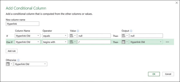
    FIGURE 2-9 You can add a conditional column as a preliminary step in adding back the domain name aka.ms. Note that the conditions in the dialog box are used as a stepping-stone to the final conditions.

    NOTE

    The use of the Add Conditional Column dialog box will help you set the stage for the final conditions. The user interface is limited, and you are using it as a shortcut to generate part of the required conditions. The final touch will require a lightweight modification of the formula in the formula bar in step 16.

    1. Enter Hyperlink in the New Column Name box.

    2. Select Hyperlink Old from the Column Name drop-down for If.

    3. Select Equals from the Operator drop-down and enter null in both the Value and Output text boxes.

    4. Click the Add Rule button to add a new condition line.

    5. Select Hyperlink Old from the Column Name drop-down for Else If.

    6. Select Begins With as the operator in the second line.

    7. Ensure that Enter a Value is selected in the ABC123 drop-down menu in the second line, under Value, and enter / in the Value box.

    8. In the drop-down menu after the Then label for Else If, select Select a Column and then select Hyperlink Old.

    9. In the drop-down menu below the Otherwise label, select Select a Column and then select Hyperlink Old.

    10. Ensure that your settings match those in Figure 2-9 and click OK to close the dialog box.

16. Now look at the formula bar. It’s time to modify the M formula to add the prefix aka.ms if a hyperlink starts with /. Here is the original formula, following step 15:

    = Table.AddColumn(#"Renamed Columns1", "Custom", each if [Hyperlink Old] = null
    then null else if Text.StartsWith([Hyperlink Old], "/") then [Hyperlink Old] else
    [Hyperlink Old])

    To fix it, you can concatenate aka.ms and [Hyperlink Old]. Much as you would do in an Excel formula, you can add aka.ms as a prefix in the Hyperlink Old column by using the & operator:

    "aka.ms" & [Hyperlink Old]

    Here is the modified formula, including the change, in bold:

    = Table.AddColumn(#"Renamed Columns1", "Custom", each if [Hyperlink Old] = null
    then null else if Text.StartsWith([Hyperlink Old], "/") then
    "aka.ms" & [Hyperlink Old] else [Hyperlink Old])

    NOTE

    In step 15, the first null condition was added to prevent Text.StartsWith from being applied on a null value in [Hyperlink Old], which would result in an error.

17. Remove the Hyperlink Old column.

    You are almost done, but there are few more surprises waiting for you. Continue auditing the results in the Hyperlink column by scrolling down to row 149. The Hyperlink cell is blank, but looking at the original Message column, you can see the following hyperlink inside the message: https://www.microsoftpressstore.com/Ignite.

    Why is the Hyperlink cell blank in this case? When you split this message in step 14, both “https://” and “www.” participated in the split as delimiters. As a result, the split included three separated values, but only the first two were loaded. The next steps help you resolve this problem.

18. In Applied Steps, select the first Split Column by Delimiter step. Change the bolded section in the formula below from {“Hyperlink.1”, “Hyperlink.2”} to 3:

    = Table.SplitColumn(#"Renamed Columns", "Hyperlink",
    Splitter.SplitTextByAnyDelimiter({"http://", "https://", "www.", "aka.ms"},
    QuoteStyle.Csv, false), {"Hyperlink.1", "Hyperlink.2"})

    Here is the complete modified formula:

    = Table.SplitColumn(#"Renamed Columns", "Hyperlink",
    Splitter.SplitTextByAnyDelimiter({"http://", "https://", "www.", "aka.ms"},
    QuoteStyle.Csv, false), 3)

    SEE ALSO

    Here you use the argument 3 instead of the list of column names {“Hyperlink.1”, “Hyperlink.2”, Hyperlink.3”}. The results are the same. The Table.SplitColumn function accepts either the column names or the number of new columns to use in the split. The fact is, you miss crucial data when you use only the default split; this is discussed in more detail in Chapter 10, “From Pitfalls to Robust Queries.”

    Now, as shown in Figure 2-10, you have the hyperlink values either in Hyperlink.2 (in most of the rows) or in Hyperlink.3 (in row 149). If you merge the two columns, you can retrieve the missing hyperlinks and fix the query.

    

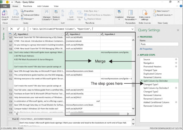
    FIGURE 2-10 You can merge the Hyperlink.2 column with the Hyperlink.3 column to extract hyperlinks that start with https://www.

19. While the Split Column by Delimiter step is still selected in Applied Steps, insert the following steps into the transformation sequence:

    1. Select the two columns Hyperlink.2 and Hyperlink.3.

    2. On the Transform tab, select Merge Columns.

    3. When the Insert Step dialog box opens, warning you that this step will be inserted between the existing steps and may break your subsequent steps, select Insert.

    4. In the Merge Columns dialog box that opens, keep the default settings and click OK to close the dialog box.

    5. Rename the Merged column Hyperlink.2.

    6. When the Insert Step dialog box opens again, select Insert.

20. You can now select the last step in Applied Steps to ensure that the preceding steps work as expected.

    There are still two cases that have not been handled correctly. First, in row 149 you can see that the hyperlinks don’t end with a space but with other punctuation, such as a dot. As a result, in step 11, when you applied space as a delimiter, you were not able to clean the trailing message from the hyperlink value. To fix it, you should trim the punctuation from all hyperlinks.

21. Select the Hyperlink column, and on the Transform tab, select Format and then select Trim. Alternatively, right-click the Hyperlink column, and in the shortcut menu, select Transform and then select Trim.

    By default, Trim removes whitespace from the beginning and end of text values. You can manipulate it to also trim the trailing punctuation. This requires some changes in the formula bar. You can see that the formula includes the bolded element Text.Trim:

    = Table.TransformColumns(#"Removed Columns1",{{"Hyperlink", Text.Trim, type text}})

    The M function Text.Trim accepts a list of text items as its second argument to trim leading and trailing text other than spaces. In M, the punctuation list—dot, comma, and closing parenthesis—can be defined with curly brackets and comma-separated double-quoted values, as shown here:

    { ".", ",", ")" }

    To feed the list as the second argument to Text.Trim, you should also feed its first argument, which is the actual text in the Hyperlink column. To get the actual text, you can use the combination of the keyword each and the underscore character. (Chapter 9 explains this in more details.) Copy this modified formula to the formula bar to trim the punctuations from the Hyperlink column:

    = Table.TransformColumns(#"Removed Columns1",{{"Hyperlink", each Text.Trim(_,
    {".",",",")"}), type text}})

22. Notice the final issue in row 174, where you can see that the hyperlink ends with a new line, followed by more text. When you applied the second Split Text By Delimiter using a space, you didn’t extract the hyperlink correctly. To fix it, select the second Split Text By Delimiter in Applied Steps.

23. In the formula bar, notice the following code:

    = Table.SplitColumn(#"Changed Type1", "Hyperlink.2",
    Splitter.SplitTextByEachDelimiter({" "}, QuoteStyle.Csv, false),
    {"Hyperlink.2.1", "Hyperlink.2.2"})

    Change it to the following (where changes are highlighted in bold):

    = Table.SplitColumn(#"Changed Type1", "Hyperlink.2",
    Splitter.SplitTextByAnyDelimiter({" ", "#(lf)"}, QuoteStyle.Csv, false),
    {"Hyperlink.2.1", "Hyperlink.2.2"})

    The value "#(lf)" describes the special line-feed character. In the preceding formula, you used the advanced split function Splitter.SplitTextByAnyDelimiter instead of Splitter.SplitTextByDelimiter to split by both spaces and line feeds.

24. Finally, to include the prefix “http://” in all the Hyperlink values, in Applied Steps, go back to the last step. Select the Hyperlink column, and on the Transform tab, select Format and then select Add Prefix. When the Prefix dialog box opens, enter “http://” in the Value box and close the dialog box.

25. In the preceding step, you added the prefix “http://” in all the rows, even where there are no URLs. But there are legitimate cases in which the Hyperlink column should be empty (for example, row 113). To remove “http://” from cells without hyperlinks, follow these steps:

    1. Select the Hyperlink column. Then, on the Home tab, select Replace Values.

    2. When the Replace Values dialog box opens, enter ”http://” in the Value to Find box.

    3. Leave the Replace With box empty.

    4. Expand Advanced Options and select the Match Entire Cell Contents check box. (This step is crucial. Without it, Power Query removes “http://” from all the values.)

    5. Click OK to close the dialog box and select Close & Load in Excel or Close & Apply in Power BI Desktop to load the messages and their extracted hyperlinks to the report.

By now, you have resolved most of the challenges in this dataset and extracted the required hyperlinks. You can download the solution files C02E04 - Solution.xlsx and C02E04 - Solution.pbix from https://aka.ms/DataPwrBIPivot/downloads.