Grouping, sorting, and filtering pivot data

By Michael Alexander and Bill Jelen
4/7/2019

Contents

Using the PivotTable Fields list
Sorting in a pivot table
Filtering a pivot table: an overview
Using filters for row and column fields
Filtering using the Filters area
Grouping and creating hierarchies in a pivot table
Creating hierarchies
Next steps

Filtering using the Filters area

Pivot table veterans remember the old Page area section of a pivot table. This area has been renamed the Filters area and still operates basically the same as in legacy versions of Excel. Microsoft did add the capability to select multiple items from the Filters area. Although the Filters area is not as showy as slicers, it is still useful when you need to replicate your pivot table for every customer.

Adding fields to the Filters area

The pivot table in Figure 4-29 is a perfect ad-hoc reporting tool to give to a high-level executive. He can use the drop-down menus in B1:B4 and E1:E4 to find revenue quickly for any combination of sector, region, market, rep, customer, product, date, or weekday. This is a typical use of filters.

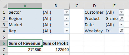
FIGURE 4-29 With multiple fields in the Filters area, this pivot table can answer many ad-hoc queries.

To set up the report, drag Revenue and Cost to the Values area and then drag as many fields as desired to the Filters area.

If you add many fields to the Filters area, you might want to use one of the obscure pivot table options settings. Click Options on the Analyze tab. On the Layout & Format tab of the PivotTable Options dialog box, change Report Filter Fields per Column from 0 to a positive number. Excel rearranges the Filter fields into multiple columns. Figure 4-29 shows the filters with four fields per column. You can also change Down, Then Over to Over, Then Down to rearrange the sequence of the Filter fields.

Choosing one item from a filter

To filter the pivot table, click any drop-down menu in the Filters area of the pivot table. The drop-down menu always starts with (All) but then lists the complete unique set of items available in that field.

Choosing multiple items from a filter

At the bottom of the Filters drop-down menu is a check box labeled Select Multiple Items. If you select it, Excel adds a check box next to each item in the drop-down menu. This enables you to select multiple items from the list.

In Figure 4-30, the pivot table is filtered to show revenue from multiple sectors, but it is impossible to tell which sectors are included.

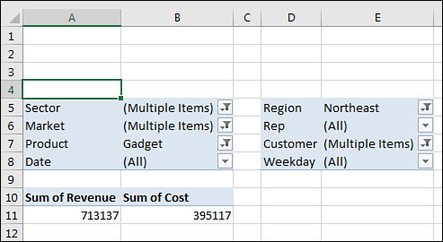
FIGURE 4-30 You can select multiple items, but after the Filter drop-down menu closes, you cannot tell which items were selected.

Replicating a pivot table report for each item in a filter

Although slicers are now the darlings of the pivot table report, the good old-fashioned report filter can still do one trick that slicers cannot do. Say you have created a report that you would like to share with the industry managers. You have a report showing customers with revenue and profit. You would like each industry manager to see only the customers in their area of responsibility.

Follow these steps to quickly replicate the pivot table:

Make sure the formatting in the pivot table looks good before you start. You are about to make several copies of the pivot table, and you don’t want to format each worksheet in the workbook, so double-check the number formatting and headings now.
Add the Sector field to the Filters area. Leave the Sector filter set to (All).
Select one cell in the pivot table so that you can see the Analyze tab in the ribbon.
Find the Options button in the left side of the Analyze tab. Next to the Options tab is a drop-down menu. Don’t click the big Options button. Instead, open the drop-down menu (see Figure 4-31).

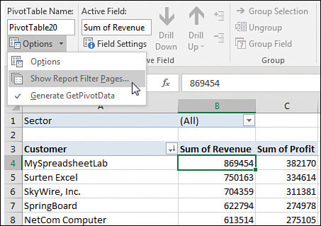
FIGURE 4-31 Click the tiny drop-down arrow next to the Options button.
Choose Show Report Filter Pages. In the Show Report Filter Pages dialog box, you see a list of all the fields in the report area. Because this pivot table has only the Sector field, this is the only choice (see Figure 4-32).

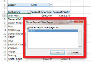
FIGURE 4-32 Select the field by which to replicate the report.
Click OK and stand back.

Excel inserts a new worksheet for every item in the Sector field. On the first new worksheet, Excel chooses the first sector as the filter value for that sheet. Excel renames the worksheet to match the sector. Figure 4-33 shows the new Consulting worksheet, with neighboring tabs that contain Museums, Retail, Training, and Utilities.

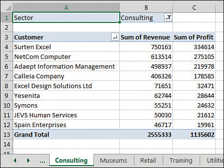
FIGURE 4-33 Excel quickly adds one page per sector.

Filtering using slicers and timelines

Slicers are graphical versions of the Report Filter fields. Rather than hiding the items selected in the filter drop-down menu behind a heading such as (Multiple Items), the slicer provides a large array of buttons that show at a glance which items are included or excluded.

To add slicers, click the Insert Slicer icon on the Analyze tab. Excel displays the Insert Slicers dialog box. Choose all the fields for which you want to create graphical filters, as shown in Figure 4-34.

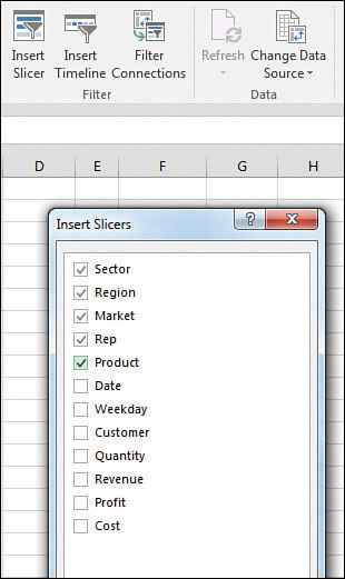
FIGURE 4-34 Choose fields for slicers.

Initially, Excel chooses one-column slicers of similar color in a cascade arrangement (see Figure 4-35). However, you can change these settings by selecting a slicer and using the Slicer Tools Options tab in the ribbon.

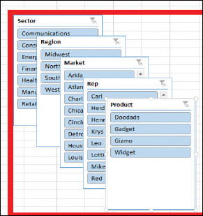
FIGURE 4-35 The slicers appear with one column each.

You can add more columns to a slicer. If you have to show 50 two-letter state abbreviations, that will look much better as 5 rows of 10 columns than as 50 rows of 1 column. Click the slicer to get access to the Slicer Tools Analyze tab. Use the Columns spin button to increase the number of columns in the slicer. Use the resize handles in the slicer to make the slicer wider or shorter. To add visual interest, choose a different color from the Slicer Styles gallery for each field.

After formatting the slicers, arrange them in a blank section of the worksheet, as shown in Figure 4-36.

FIGURE 4-36 After formatting, your slicers might fit on a single screen.

Three colors might appear in a slicer. The dark color indicates items that are selected. Gray boxes often mean the item has no records because of other slicers. White boxes indicate items that are not selected.

Note that you can control the heading for the slicer and the order of items in the slicer by using the Slicer Settings icon on the Slicer Tools Options tab of the ribbon. Just as you can define a new pivot table style, you can also right-click an existing slicer style and choose Duplicate. You can change the font, colors, and so on.

A new icon debuted in Excel 2016, in the top bar of the slicer. The icon appears as three check marks. When you select this icon, you can select multiple items from the slicer without having to hold down the Ctrl key.

Using timelines to filter by date

After slicers were introduced in Excel 2010, there was some feedback that using slicers was not an ideal way to deal with date fields. You might end up adding some fields to your original data set to show (perhaps) a decade and then use the group feature for year, quarter, and month. You would end up with a whole bunch of slicers all trying to select a time period, as shown in Figure 4-37.

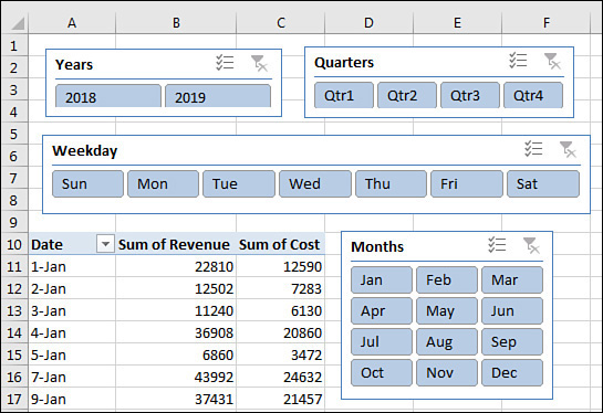
FIGURE 4-37 Four different slicers are necessary to filter by date.

For Excel 2013, Microsoft introduced a new kind of filter called a Timeline slicer. To use one, select one cell in your pivot table and choose Insert Timeline from the Analyze tab. Timeline slicers can only apply to fields that contain dates. Excel gives you a list of date fields to choose from, although in most cases, there is only one date field from which to choose.

Figure 4-38 shows a Timeline slicer. Perhaps the best part of a Timeline slicer is the drop-down menu that lets you repurpose the timeline for days, months, quarters, or years. This works even if you have not grouped your daily dates up to months, quarters, or years.

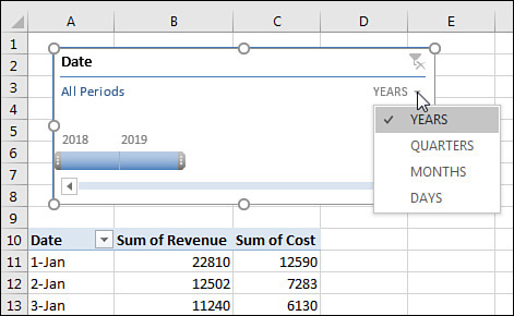
FIGURE 4-38 A single Timeline slicer can filter your pivot table by month, quarter, year, or day.

Driving multiple pivot tables from one set of slicers

Chapter 12, “Enhancing pivot table reports with macros,” includes a tiny macro that lets you drive two pivot tables with one set of filters. This has historically been difficult to do unless you used a macro.

Now, one set of slicers or timelines can be used to drive multiple pivot tables or pivot charts. In Figure 4-39, the Market slicer is driving three elements. It drives the pivot table in the top left with revenue by sector and product. It drives two pivot tables created for the top-right and lower-left charts.

FIGURE 4-39 Three pivot elements controlled by the same slicer.

The following steps show you how to create three pivot tables that are tied to a single slicer:

Create your first pivot table.
Select a cell in the first pivot table. Choose Insert Slicer. Choose one or more fields to be used as a slicer. Alternatively, insert a Timeline slicer for a date field.
Select the entire pivot table.
Copy with Ctrl+C or the Copy command.
Select a new blank area of the worksheet.
Paste. Excel creates a second pivot table that shares the pivot cache with the first pivot table. In order for one slicer to run multiple pivot tables, they must share the same pivot cache.
Change the fields in the second pivot table to show some other interesting analysis.
Repeat steps 3–7 to create a third copy of the pivot table.

The preceding steps require you to create the slicer after you create the first pivot table but before you make copies of the pivot table.

If you already have several existing pivot tables and need to hook them up to the same slicer, follow these steps:

Click the slicer to select it. When the slicer is selected, the Slicer Tools Design tab of the ribbon appears.
Select the Slicer Tools Design tab and choose Report Connections. Excel displays the Report Connections (Market) dialog box. Initially, only the first pivot table is selected.
As shown in Figure 4-40, choose the other pivot tables in the dialog box and click OK.

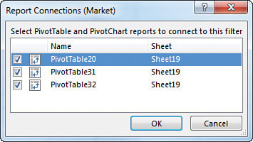
FIGURE 4-40 Choose to hook this slicer up to the other pivot tables.
If you created multiple slicers and/or timelines, repeat steps 1 through 3 for the other slicers.