Grouping, sorting, and filtering pivot data

- By Michael Alexander and Bill Jelen
- 4/7/2019
In this sample chapter from Microsoft Excel 2019 Pivot Table Data Crunching, you will review the PivotTable Fields list and then learn how to how to group, sort, and filter data.
With Excel 2019, Microsoft has reversed the auto date grouping added to Excel 2016. Removing the feature was a good move, as the feature proved hard to predict. For anyone who loved the auto grouping and the Drill-Down and Drill-Up features, you can re-create them, although it requires a few extra steps. Grouping will be covered last in this chapter.
First, a quick overview of the PivotTable Fields. Then, a detailed look at sorting, filtering, and grouping a pivot table.
Using the PivotTable Fields list
The entry points for sorting and filtering are spread throughout the Excel interface. It is worth taking a closer look at the row header drop-downs and the PivotTable Fields list before diving in to sorting and filtering.
As you’ve seen in these pages, I rarely use the Compact form for a pivot table. I use Pivot Table Defaults to make sure my pivot tables start in Tabular layout instead of Compact layout. Although there are many good reasons for this, one is illustrated in Figures 4-1 and 4-2.
)
)
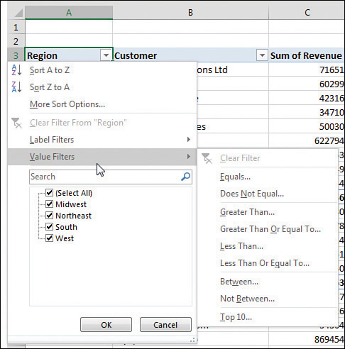
FIGURE 4-1 The drop-down menu in B3 for Customer is separate from the drop-down menu for Region.
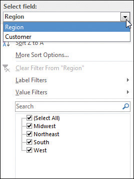
FIGURE 4-2 In Compact form, one single drop-down menu tries to control sorting and filtering for all the row fields.
In Figure 4-1, a Region drop-down menu appears in A3. A Customer drop-down menu appears in B3. Each of these separate drop-downs offers great settings for sorting and filtering.
When you leave the pivot table in the Compact form, there are not separate headings for Region and Customer. Both fields are crammed into column A, with the silly heading Row Labels. This means the drop-down menu always offers sorting and filtering options for Region. Every time you go back to the A3 drop-down menu with hopes of filtering or sorting the Customer field, you have to reselect Customer from a drop-down at the top of the menu. This is an extra click. If you are making five changes to the Customer field, you are reselecting Customer over and over and over and over and over. This should be enough to convince you to abandon the Compact layout.
If you decide to keep the Compact layout and get frustrated with the consolidated Row Labels drop-down menu, you can directly access the invisible drop-down menu for the correct field by using the PivotTable Fields list, which contains a visible drop-down menu for every field in the areas at the bottom. Those visible drop-down menus do not contain the sorting and filtering options.
The good drop-down menus are actually in the top of the Fields list, but you have to hover over the field to see the drop-down menu appear. After you hover as shown in Figure 4-3, you can directly access the same customer drop-down menu shown in Figure 4-1.
)
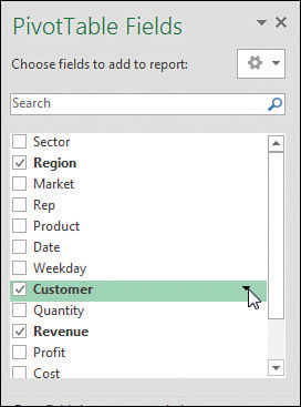
FIGURE 4-3 Hover over the field in the top of the Fields list to directly access the sorting and filtering settings for that field.
Docking and undocking the PivotTable Fields list
The PivotTable Fields list starts out docked on the right side of the Excel window. Hover over the green PivotTable Fields heading in the pane, and the mouse pointer changes to a four-headed arrow. Drag to the left to enable the pane to float anywhere in your Excel window.
After you have undocked the PivotTable Fields list, you might find that it is difficult to redock it on either side of the screen. To redock the Fields list, you must grab the title bar and drag until at least 85% of the Fields list is off the edge of the window. Pretend that you are trying to remove the floating Fields list completely from the screen. Eventually, Excel gets the hint and redocks it. Note that you can dock the PivotTable Fields list on either the right side or the left side of the screen.
Rearranging the PivotTable Fields list
As shown in Figure 4-4, a small gear-wheel icon appears near the top of the PivotTable Fields list. Select this drop-down menu to see its five possible arrangements. Although the default is to have the Fields section at the top of the list and the Areas section at the bottom of the list, four other arrangements are possible. Other options let you control whether the fields in the list appear alphabetically or in the same sequence that they appeared in the original data set.
)
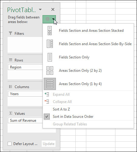
FIGURE 4-4 Use this drop-down menu to rearrange the PivotTable Fields list.
The final three arrangements offered in the drop-down menu are rather confusing. If someone changes the PivotTable Fields list to show only the Areas section, you cannot see new fields to add to the pivot table.
If you ever encounter a version of the PivotTable Fields list with only the Areas section (see Figure 4-4) or only the Fields section, remember that you can return to a less-confusing view of the data by using the arrangement drop-down menu.
Using the Areas section drop-downs
As shown in Figure 4-5, every field in the Areas section has a visible drop-down arrow. When you select this drop-down arrow, you see four categories of choices:
)
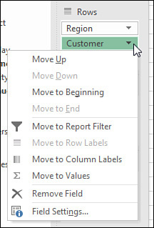
FIGURE 4-5 Use this drop-down menu to rearrange the fields in your pivot table.
The first four choices enable you to rearrange the field within the list of fields in that area of the pivot table. You can accomplish this by dragging the field up or down in the area.
The next four choices enable you to move the field to a new area. You could also accomplish this by dragging the field to a new area.
The next choice enables you to remove the field from the pivot table. You can also accomplish this by dragging the field outside the Fields list.
The final choice displays the Field Settings dialog box for the field.