Grouping, sorting, and filtering pivot data

Using filters for row and column fields

If you have a field (or fields) in the row or column area of a pivot table, a drop-down menu with filtering choices appears on the header cell for that field. In Figure 4-16, a Customer drop-down menu appears in A4, and a Product drop-down menu appears in B3. The pivot table in that figure is using Tabular layout. If your pivot tables use Compact layout, you see a drop-down menu on the cell with Row Labels or Column Labels.

If you have multiple row fields, it is just as easy to sort using the invisible drop-down menus that appear when you hover over a field in the top of the PivotTable Fields list.

Filtering using the check boxes

You might have a few annoying products appear in a pivot table. In the present example, the Doodads product line is a specialty product with very little sales. It might be an old legacy product that is out of line, but it still gets an occasional order from the scrap bin. Every company seems to have these orphan sales that no one really wants to see.

The check box filter provides an easy way to hide these items. Open the Product drop-down menu and clear the Doodads check box. The product is hidden from view (see Figure 4-17) .

FIGURE 4-17 Open the Product filter and clear the Doodads check box.

What if you need to clear hundreds of items’ check boxes in order to leave only a few items selected? You can toggle all items off or on by using the Select All check box at the top of the list. You can then select the few items that you want to show in the pivot table.

In Figure 4-18, Select All turned off all customers and then two clicks reselected Excel4Apps and F-Keys Ltd.

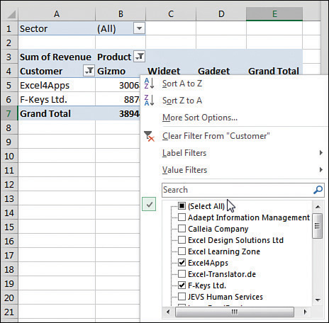
FIGURE 4-18 Use Select All to toggle all items off or on.

The check boxes work great in this tiny data set with 26 customers. In real life, with 500 customers in the list, it will not be this easy to filter your data set by using the check boxes.

Filtering using the search box

When you have hundreds of customers, the search box can be a great timesaver. In Figure 4-19, the database includes consultants, trainers, and other companies. If you want to narrow the list to companies with Excel or spreadsheet in their name, you can follow these steps:

1. Open the Customer drop-down menu.

2. Type Excel in the search box (see Figure 4-19).

   

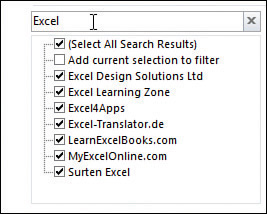
   FIGURE 4-19 Select the results of the first search.

3. By default, Select All Search Results is selected. Click OK.

4. Open the Customer drop-down menu again.

5. Type spreadsheet in the search box.

6. Choose Add Current Selection to Filter, as shown in Figure 4-20. Click OK.

   

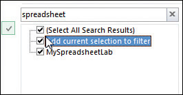
   FIGURE 4-20 For the second search, add these results to the existing filter.

You now have all customers with either Excel or spreadsheet in the name.

Filtering using the Label Filters option

The search box isn’t perfect. What if you want to find all the Lotus 1-2-3 consultants and turn those off? There is no Select Everything Except These Results choice. Nor is there a Toggle All Filter Choices choice. However, the Label Filters option enables you to handle queries such as “select all customers that do not contain ‘Lotus.’”

Text fields offer a flyout menu called Label Filters. To filter out all of the Insurance customers, you can apply a Does Not Contain filter (see Figure 4-21). In the next dialog box, you can specify that you want customers that do not contain Excel, Exc, or Exc* (see Figure 4-22).

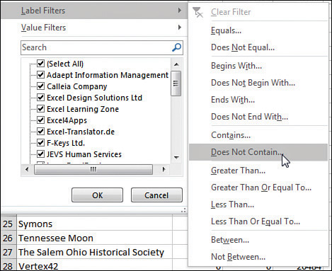
FIGURE 4-21 Choose Label Filters, Does Not Contain.

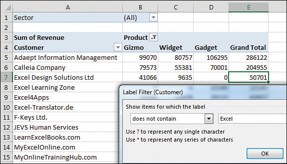
Figure 4-22 Specify to exclude customers containing Excel.

Note that label filters are not additive. You can only apply one label filter at a time. If you take the data in Figure 4-21 and apply a new label filter of between D and Fzzz, some Excel customers that were filtered out in Figure 4-22 come back, as shown in Figure 4-23.

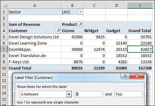
FIGURE 4-23 Note that a second label filter does not get added to the previous filter. Excel is back in.

Filtering a Label column using information in a Values column

The Value Filters flyout menu enables you to filter customers based on information in the Values columns. Perhaps you want to see customers who had between $20,000 and $30,000 of revenue. You can use the Customer heading drop-down menu to control this. Here’s how:

1. Open the Customer drop-down menu.

2. Choose Label Filters.

3. Choose Between (see Figure 4-24).

   

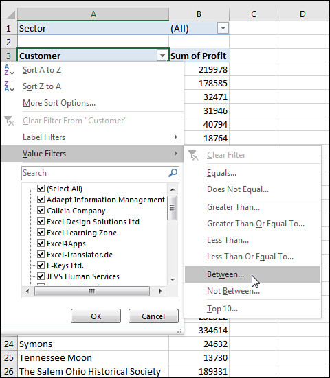
   Figure 4-24 Value Filters for the Customer column will look at values in the Revenue field.

4. Type the values 20000 and 30000, as shown in Figure 4-25.

   

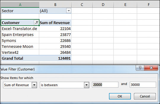
   FIGURE 4-25 Choose customers between 20000 and 30000, inclusive.

5. Click OK.

The results are inclusive; if a customer had exactly $20,000 or exactly $30,000, they are returned along with the customers between $20,000 and $30,000.

Creating a top-five report using the Top 10 filter

One of the more interesting value filters is the Top 10 filter. If you are sending a report to the VP of Sales, she is not going to want to see hundreds of pages of customers. One short summary with the top customers is almost more than her attention span can handle. Here’s how to create it:

1. Go to the Customer drop-down menu and choose Value Filters, Top 10.

2. In the Top 10 Filter dialog box, which enables you to choose Top or Bottom, leave the setting at the default of Top.

3. In the second field, enter any number of customers: 10, 5, 7, 12, or something else.

4. In the third drop-down menu on the dialog box, select from Items, Percent, and Sum. You could ask for the top 10 items. You could ask for the top 80% of revenue (which the theory says should be 20% of the customers). Or you could ask for enough customers to reach a sum of $5 million (see Figure 4-26).

   

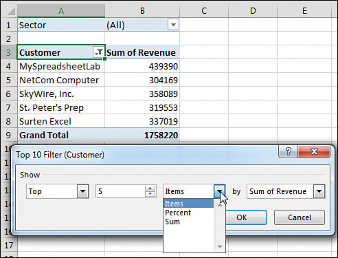
   FIGURE 4-26 Create a report of the top five customers.

The $1,758,220 total shown in cell B9 in Figure 4-26 is the revenue of only the visible customers. It does not include the revenue for the remaining customers. You might want to show the grand total of all customers at the bottom of the list. You have a few options:

• A setting on the Design tab, under the Subtotals drop-down menu, enables you to include values from filtered items in the totals. This option is available only for OLAP data sets and data sets where you choose Add This Data To The Data Model when creating the pivot table.

• You can remove the grand total from the pivot table in Figure 4-27 and build another one-row pivot table just below this data set. Hide the heading row from the second pivot table, and you will appear to have the true grand total at the bottom of the pivot table.

  

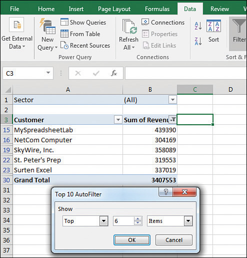
  FIGURE 4-27 You are taking advantage of a hole in the fabric of Excel to apply a regular AutoFilter to a pivot table.

• If you select the blank cell to the right of the last heading (C3 in Figure 4-26), you can turn on the filter on the Data tab. This filter is not designed for pivot tables and is usually grayed out. After you’ve added the regular filters, open the drop-down menu in B3. Choose Top 10 Filter and ask for the top six items, as shown in Figure 4-27. This returns the top five customers and the grand total from the data set.

Filtering using the Date filters in the Label drop-down menu

If your label field contains all dates, Excel replaces the Label Filter flyout with a Date Filters flyout. These filters offer many virtual filters, such as Next Week, This Month, Last Quarter, and so on (see Figure 4-28).

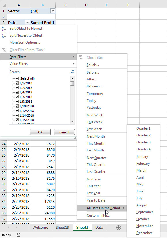
FIGURE 4-28 The Date Filters menu offers various virtual date periods.

If you choose Equals, Before, After, or Between, you can specify a date or a range of dates.

Options for the current, past, or next day, week, month, quarter, or year occupy 15 options. Combined with Year To Date, these options change day after day. You can pivot a list of projects by due date and always see the projects that are due in the next week by using this option. When you open the workbook on another day, the report recalculates.

When you select All Dates In The Period, a new flyout menu offers options such as Each Month and Each Quarter.