Grouping, sorting, and filtering pivot data

By Michael Alexander and Bill Jelen
4/7/2019

Contents

Using the PivotTable Fields list
Sorting in a pivot table
Filtering a pivot table: an overview
Using filters for row and column fields
Filtering using the Filters area
Grouping and creating hierarchies in a pivot table
Creating hierarchies
Next steps

Filtering a pivot table: an overview

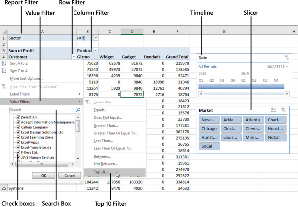
Excel 2019 provides dozens of ways to filter a pivot table. Figure 4-16 shows some of the filters available. These methods, and the best way to use each one, are discussed in the following sections.

FIGURE 4-16 This figure shows a fraction of the available filtering choices.

There are four ways to filter a pivot table, as shown in Figure 4-16:

The Date Timeline filter in G4:H10 was introduced in Excel 2013.
The Market filter in G12:H19 is an example of the slicer introduced in Excel 2010.
A drop-down menu in B1 offers what were known as page filters in Excel 2003, report filters in Excel 2010, and now simply filters.
Cell G4 offers the top-secret AutoFilter location.
Drop-down menus in A4 and B3 lead to even more filters.
You see the traditional check box filters for each pivot item.
A Search box filter was introduced in Excel 2010.
A flyout menu has Label filters.
Depending on the field type, you might see a Value Filters flyout menu, including the powerful Top 10 filter, which can do Top 10, Bottom 5, Bottom 3%, Top $8 Million, and more.
Depending on the field type, you might see a Date Filters flyout menu, with 37 virtual filters such as Next Month, Last Year, and Year to Date.