Use other services for machine learning
- By Julio Granados and Ginger Grant
- 4/11/2018
- Skill 4.1: Build and use neural networks with the Microsoft Cognitive Toolkit
- Skill 4.2: Streamline development by using existing resources
- Skill 4.3: Perform data science at scale by using HDInsight
- Skill 4.4: Perform database analytics by using SQL Server R Services on Azure
- Thought experiment
- Thought experiment answers
- Chapter summary
Skill 4.4: Perform database analytics by using SQL Server R Services on Azure
Developing or even trying out a data science solution can be a resource-intensive task. Many machine learning algorithms, given moderately sized datasets, will take from minutes to hours to train, and if you add this basic delay to an iterative process where you need to visually explore variables, perform statistical tests, and transformations on the dataset and tune algorithm parameters, coming up with a production level model becomes quite time consuming.
In order to minimize development time, minimize architecture/hardware maintenance, and quickly scale up resources in case bulkier algorithms need them, or scale down if the resources are no longer needed, Microsoft offers quickly deployable Virtual Machines on Azure. Some of the major benefits of hosting both an application and the data within Azure is that you automatically can rely on the multiple global datacenters in order to distribute computation, have replicated instances for disaster recovery, or just for load balancing workloads across different resources.
In Skill 4.1 of this book you have configured and worked on the Data Science Virtual Machine,, which comes preloaded with an arsenal of data science tools that enable you to develop anything from a deep learning application to simple graphic interface machine learning solutions in Weka. However, what if you do not require nor are you willing to pay for all those extra resources, while requiring an in-database machine learning service?
Under such scenarios, there is the option of deploying a SQL Server Azure Virtual Machine (SQLVM). The SQL Server Azure Virtual Machine offers a cheaper alternative as compared to the Data Science Virtual Machine, mainly because of the missing associated software plans costs of the DSVM. The advantage of the SQLVM is that, as you see below, the latest versions of SQL Server, SQL Server 2016 and SQL Server 2017, both come with associated R and Machine Learning services, which enables the development of machine learning solutions. These solutions, which are based on R and Python, can be directly executed either from traditional R and Python development environments, or from SQL Server Management Studio as stored procedures close to the relational data. Other advantages of the SQLVM stems directly from the benefits of using an in-database machine learning service: less data movement, real time scoring, TSQL language to process data, columnar storage, and binary model storage and a TSQL PREDICT clause to embed predictions in your queries.
Other reasons to deploy a SQL Virtual Machine come closely associated with why you would move your applications and databases to the cloud. The main two reasons are interoperability and availability: with an Azure SQL Virtual Machine your data will always be backed up, and with high availability in case a server is out of service. As for interoperability, you can easily connect your SQL VM to many other Azure services and amplify the features that are part of your machine learning solution.
Currently there are four machine-learning services available with SQL Server distributions. The name and full features depend on the version of SQL Server deployed:
SQL Server 2016 R Services (In-Database) This is the initial service version offered with SQL Server 2016 Developer and Enterprise. It incorporates the RevoScaleR functions for faster parallel and distributed R processing, the MicrosoftML algorithms, which perform better than many industry leading algorithms, and an array of R API calls to Cortana Intelligence to complement your R solutions with the Cortana services.
SQL Server 2017 Machine Learning Services (In-Database) The main addition to the SQL Server 2017 Machine Learning Services is the Python Services, which have been developed similarly to the R Services: The incorporate a RevoScalePy library for parallel and distributed Python computing, as well as the MicrosoftML library with its added functionality.
Standalone Machine Learning Server This is an optional install when you already have an instance of SQL Server 2016 or SQL Server 2017 installed without R or Machine Learning Services. Essentially, you are able to install the services as standalone software, and then link them to your already existing instance.
Azure SQL Databases Some Azure regions are starting to support the execution of R scripts and the use of the PREDICT command. Python and MicrosoftML is not yet supported.
Deploy a SQL Server 2016 Azure VM
In this section you review how to deploy a SQL Server Azure VM from the portal, configure and connect to it for its further use in developing R and Python machine learning solutions closely associated to a SQL Server and its databases.
Types of Azure VMs
When deciding upon a type of virtual machine for your machine learning solution needs, you first need to consider which version of SQL Server you need. As discussed before, the main difference between the versions is that SQL Server 2017 enables you to develop Python-based solutions in addition to R-based solutions, whereas on SQL Server 2016 you are only able to develop R-based solutions. In addition, SQL Server 2017 comes with a Machine Learning Python library called MicrosoftML. The library has deep pretrained models (like ResNet and AlexNet) that you can easily use for image featurization. Other functionalities such as text featurization and sentiment analysis are also available in the library.
You could deploy SQL Server on a Linux operating system as well, but there are some hurdles to developing SQL R Services related solutions. The current distribution of SQL Server 2017 for Linux does not include in-database R Services, thus if you are a data scientist used to the Linux environment and you wish to use this feature natively on Linux, currently you will not be able to do it. However, you could always deploy SQL Server 2017 on Windows virtual machine hosted on you Linux system, wherein you will be able to use the full features of the Windows SQL Server 2017 that are not yet included in the Linux SQL Server 2017, such as R Services, to Analysis Services and Reporting Services.
Finally, you have to decide the hardware that best suits your needs. As of late 2017 there are six families of virtual machines (https://docs.microsoft.com/en-us/azure/virtual-machines/windows/sizes), each aiming to satisfy a particular type of computation task:
General Purpose Virtual machines with a balanced CPU-to-memory ratio. Ideal for testing and development, for small to medium databases and low to medium web traffic. The following machines fall under this category: B (Preview), Dsv3, Dv3, DSv2, Dv2, DS, D, Av2, A0-7.
Compute Optimized Virtual machines with a higher CPU-to-memory ratio. Ideal for medium web traffic, network appliances, batch processes, and application servers. The following machines fall under this category: Fsv2, Fs, F.
Memory Optimized Virtual machines with a high memory-to-CPU ratio. Ideal for relational databases, in-memory cubes, models and analytics. The following machines fall under this category: Esv3, Ev3, M, GS, G, DSv2, DS, Dv2, D.
Storage optimized Virtual machines ideal for disk IO intensive operations, such as big data, SQL, and NoSQL databases. The following machines fall under this category: Ls.
GPU Enabled Specialized virtual machines with GPUs ideal for heavy graphic rendering, video editing, and deep learning solutions. The following machines fall under this category: NV, NC.
High performance compute Virtual machines with the fastest and most powerful CPUs available in the datacenter. Ideal for high-throughput, real time, and big data applications. The following machines fall under this category: H, A8-11.
Create an Azure VM
You will deploy, configure, and use a SQL Server 2017 Developer on Windows Server 2016 Standard_A4_v2 virtual machine in the rest of this chapter. This machine offers a fully featured free option for developing and testing R and Python solutions associated to a SQL Server and its databases because of the SQL developer edition installed with the machine. The hardware choice stems from it being one of the newest general-purpose machines, with a slight balance toward higher memory for handling moderately sized datasets in R and Python.
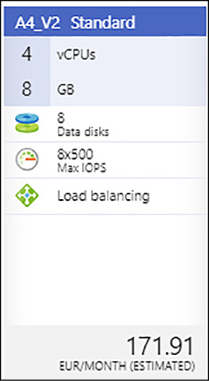
FIGURE 4-53 Suggested Virtual Machine Configuration
First, log in to the Azure Portal using your account (https://portal.azure.com/). Once the portal launches, click the Create Resource plus sign, click the Compute resources, and then click the See All option, as shown in Figure 4-54.
)
FIGURE 4-54 Azure Portal resource creation
If you cannot see the Free SQL Server License: SQL Server 2017 Developer On Windows Server 2016 virtual machine, search for Free SQL Server 2017 in the search box, and click the indicated virtual machine, as shown in Figure 4-55.
)
FIGURE 4-55 Azure SQL Virtual Machines
SQL Server virtual machine images include the licensing costs for SQL Server (and other deployed software, as in the case of the DSVM) into the per-minute pricing of the VM you create. SQL Server Developer and Express editions are exceptions because their SQL licensing costs are zero. SQL Server Developer is a fully featured SQL Server used for development and testing (not to be used in production). SQL Express is meant for lightweight environments and workloads, with a maximum of 1 GB of memory allocation and a maximum of 10 GBs of storage size. Another exception are the Bring Your Own License (BYOL) SQL Server machines. Those VM images will not include licensing costs, you only must acknowledge that you have a valid SQL Server Enterprise license.
After choosing the virtual machine, you are directed to a general description of the machine, along with links for further information on documentation, SQL Server 2017, and pricing terms. Click Create, leaving the option of selecting a deployment model to its default, Resource Manager.
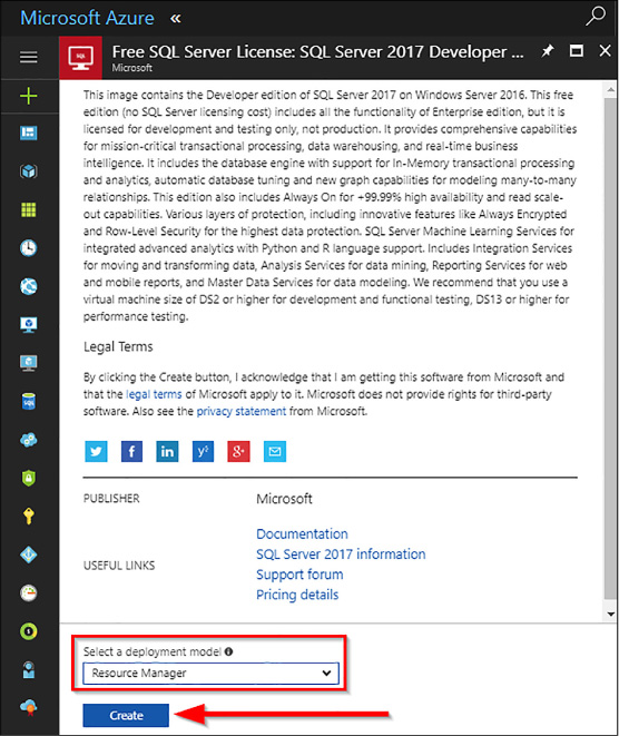
FIGURE 4-56 VM deployment confirmation
Configure an Azure VM
After you create the selected VM, you have five final steps to configure the VM:
Basics Configure basic settings.
Size Choose virtual machine size.
Settings Configure optional features.
SQL Server Settings Configure SQL Server settings.
Summary Check that everything is correct before deploying.
Configure basic settings
Under the Basics tab, you are required to input the following values and configurations:
Enter a name for your VM. Remember that only lowercase names with dashes are accepted.
Select either SSD of HDD for your virtual machine. If you wish to deploy any of the Av2 family, select HDD as the VM disk type. Those machines are not recommended for SQL production workloads, but are good for this demo because they are cheaper.
Create a user name for your VM. This user will be the administrator account for the VM, and it will be added as an SQL Server sysadmin login.
Specify a password for the user name.
Select the subscription under which you wish to deploy the VM.
Associate your VM to either an existing or a new user group. A resource group is a collection of related Azure resources, generally belonging to the same solution or application.
Select a Location that will host your VM. As a rule of thumb, you should select the datacenter nearest to your current client or development PC. Also, take a look at the price estimator, for sometimes the same VM might be slightly cheaper in another datacenter.
Click OK to save the settings.
)
FIGURE 4-57 Virtual Machine Basics settings
Configure the VM size
The next step is to configure the VM size. On the Size step, select which virtual machine hardware you wish to deploy. The Choose A Size blade displays recommended sizes based on the selected image to be deployed. Browse all the other available sizes and select one suited to your necessities, or if the purpose is only following this chapter, select the Standard_A4_v2 virtual machine. The estimated monthly cost includes SQL Server and other software licensing costs. However, because you are deploying a free SQL Server Developer Edition with no licensing cost, the cost displayed equals that of the maintenance of the VM alone; this estimated cost will also be the total monthly cost of our deployment.
Choose the machine size and click Select, as shown in Figure 4-58.
)
FIGURE 4-58 Choose a size for your VM Pane
Configure optional features
The next step in the VM configuration is the configuration of optional features. These include High Availability, Storage Management, Network Settings, Extensions, Auto-shutdown, and Monitoring options. See Figure 4-59 for an example.
Specify the desired availability set of your VM. Availability sets are managed groups of VMs that are ensured to provide at least one available VM from the group in case of a planned or unplanned maintenance event. Leave this options to None.
Confirm the Storage mode to use managed disks. Managed disks automatically handle storage accounts, availability, and scaling in case the machine needs to be rescaled.
Network settings are used to configure the VMs virtual network, subnet, Public IP visibility, firewall security group, and accelerated throughput on the VM network interface. Leave all the options to the defaults specified.
Extensions allow you to add additional software to your VM, such as antiviruses or backup suites. Leave this option to None.
Enable the auto-shutdown if you wish to schedule the shutdown of the VM in order to save on resource consumption. Click On, and select a shutdown time and time zone.
The Monitoring option comes enabled by default. Azure uses the same storage account for monitoring as the one the VM is based on.
Click OK to save the settings.
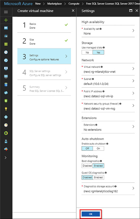
FIGURE 4-59 VM Optional Configuration pane
Configure SQL Server settings
In this step, you configure SQL Server settings, optimizations, access, and other management settings of SQL Server. Refer to Figure 4-59 as an example.
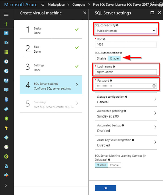
FIGURE 4-60 VM SQL Server Settings
Under the SQL Connectivity option, you can specify the type of access you want to the SQL server instance in your VM. You have three options:
Local (inside VM only) to allow connections to SQL Server only from within the VM.
Private (within Virtual Network) to allow connections to SQL Server from machines or services in the same virtual network.
Public (Internet)
For the purposes of this chapter, select Public (Internet) to allow connections to SQL Server from machines or services on the Internet. Once this option is selected, Azure automatically configures the firewall and the network security group.
In order to connect to your SQL Server instance from outside your VM, you must also enable SQL Authentication. Once enabled, you will be able to specify a different SQL Server admin and password to the default. Otherwise, Azure uses the same user and password as the one for the VM. This user is created with a sysadmin server role. If you do not enable SQL Server Authentication, you can use the VM Administrator account to connect to the SQL Server instance.
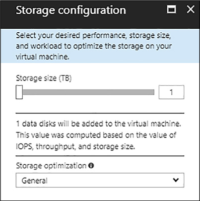
FIGURE 4-61 SQL Server Storage Configuration blade
Under the Storage Configuration blade (Figure 4-60), you are able to configure the SQL Server storage requirements. You can specify requirements as input/output operations per second, throughput in MB/s, and total storage size. You can change these settings based on workload. Azure automatically calculates the number of disks to attach and configure based on these requirements.
Under Storage Optimized For, select one of the following options:
General is the default setting and supports most workloads.
Transactional processing optimizes the storage for traditional database OLTP workloads.
Data warehousing optimizes the storage for analytic and reporting workloads.
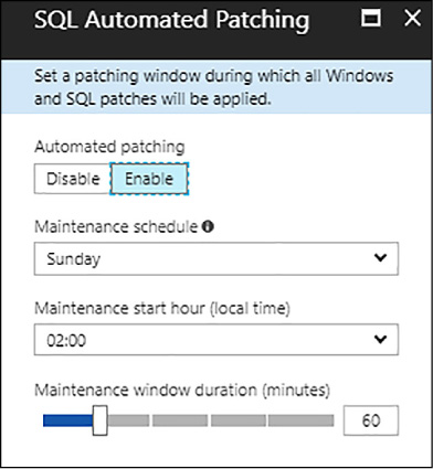
FIGURE 4-62 SQL Automated Patching blade
Automatic Patching is enabled by default, as shown in Figure 4-61. It allows Azure to automatically patch SQL Server and the operating system. You should specify the scheduled time for maintenance, as well as the window duration.
Under the automated Backup window, as shown in Figure 4-62, you are able to configure the backup policies of you SQL Server instance. As you click enable, you will be able to configure:
Retention period (days) for backups
Storage account to use for backups
Encryption option and password for backups
Backup system databases
Configure backup schedule
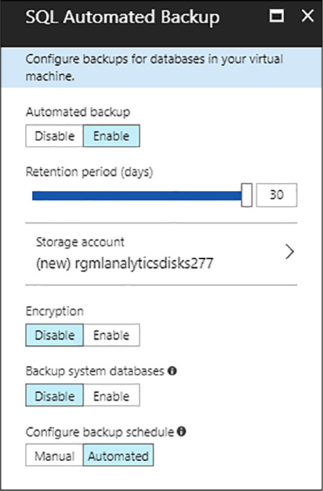
FIGURE 4-63 SQL Automated Backup blade
Continuing with the SQL Server configuration, as shown in Figure 4-59, Azure Key Vault integration allows your VM to connect to the Azure Key Vault service for a cloud-based key storage. Leave this option disabled.
Finally, SQL Server Machine Learning services allows you to install the latest machine learning service with your SQL Server 2017 Developer edition installation. Leave this option enabled.
Once finished click OK to continue
Summary pane
On the summary blade, you are able to review the configuration for your SQL 2017 VM and confirm its creation. If this is a reiterated deployment, you can download the template and parameters and deploy similar machines without having to go through the whole setup process. Once you reviewed the settings, click Create.

FIGURE 4-64 Summary Confirmation blade
Connect to VMs with RDP
In order to connect to your VM, once it is created, open it within the Azure Portal, as shown in Figure 4-64. On the upper bar of the Virtual Machine window you will find the Connect option. Click it and a RDP file is downloaded. Open the RDP file, on the Remote Desktop Connection click Connect, and then change your credentials to use the admin and password specified during setup, as shown in Figure 4-65. Click OK to connect to the VM.
)
FIGURE 4-65 Azure Portal Virtual Machine Summary
After you connect to the SQL Server virtual machine, you can launch SQL Server Management Studio and connect with Windows Authentication using your local administrator credentials. If you enabled SQL Server Authentication, you can also connect with SQL Authentication using the SQL login and password you configured during provisioning.
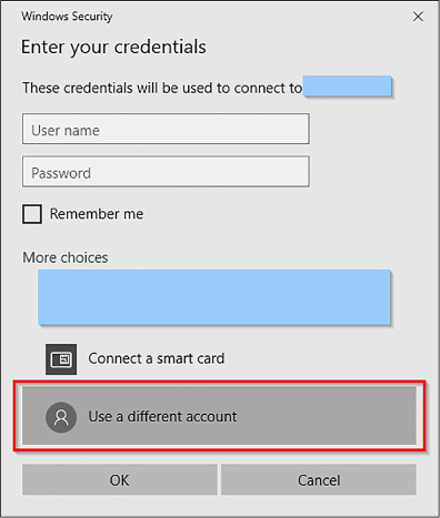
FIGURE 4-66 Connect to the Virtual Machine using your credentials
Access to the machine enables you to directly change machine and SQL Server settings based on your requirements. For example, you could configure the firewall settings or change SQL Server configuration settings.
Connect to SQL Server remotely
Previously you configured a Public access for the virtual machine and SQL Server Authentication when deploying the virtual machine. By enabling these two settings, you can connect to the VM’s SQL Server instance from outside the virtual machine, by using any client you choose as long as you have the correct SQL login and password. Before being able to do so, you need to enable a couple of features in your VM settings.
Configure a DNS label for the public IP address.
Login into your Azure Portal and open your Virtual Machine configurations page. Click DNS Name on the right hand side of your settings summary. A Configuration blade will show up, as shown in Figure 4-67.
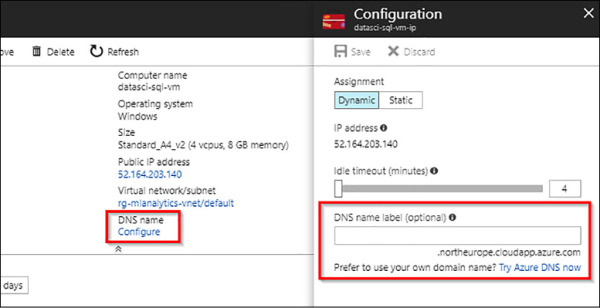
FIGURE 4-67 Setup the DNS name for your virtual machine
Enter a DNS Label name. This will be the “readable” Internet address of your virtual machine. Save the full address to a known location, and click Save.
Connect to the database engine from another computer.
Open SQL Server Management Studio (SSMS), and on the Connect To Server dialog box, specify the DNS Label name you just set up for the VM IP address. Type in the virtual machine login and password (or SQL Server login and password, if different from the main administrator account for the virtual machine), and click Connect.
)
)
FIGURE 4-68 Connect to the Server Window
In the event that SQL Server Management Studio refuses to connect due to The Certificate Chain Was Issued By An Authority That Is Not Trusted, click Options, and enable the ‘Trust Server Certificate’ option, as shown in Figure 4-69. This is just an example, but keep in mind that relying on a certificate not issued by an authority implies security problems.
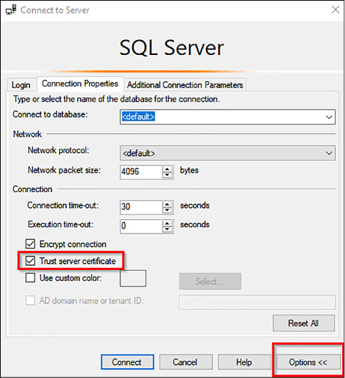
FIGURE 4-69 Additional Connect To Server options
Configure SQL Server to allow execution of R scripts
The deployed VM has all the required configurations in order to run R scripts from a query window right from the start. However, depending on your use case for Machine Learning Services you might need to make additional changes and configure the server, firewall, accounts, or database/server permissions.
A few common scenarios that require you to change internal configurations are:
Verify and configure execution of R scripts
Unblock the firewall
Enable ODBC callbacks for remote clients
Enabling additional network protocols
Enable TCP/IP for Developer and Express editions
Add more worker accounts
Ensuring that users have permission to run code or install packages
Install Additional R packages
Verify and configure execution of R scripts
You must always carry out this step before using either R Services or Machine Learning Services because this is one of the most important configurations/checks. Open your connection to the virtual machine and execute the following command:
sp_configure
Check that the run_value for the external scripts enabled property is set to 1. Verify in the SQL Server Configuration Manager, SQL Server Services that the SQL Server Launchpad is running. In order to verify that SQL can run R Scripts, run the following code:
EXEC sp_execute_external_script  @language =N'R',
@script=N'
OutputDataSet <- InputDataSet;',
@input_data_1 =N'SELECT 1 AS hello'
WITH RESULT SETS (([hello] int not null));
GO
If your machine is configured correctly, you should see the following output (Figure 4-70):
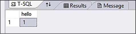
FIGURE 4-70 Correct output from executing the Hello TSQL R script
However, if your results are different from the above, you need to enable the execution of external scripts. In order to do so, execute the following code with an account that has owner permissions at the instance level (the VM account has these permissions):
sp_configure 'external scripts enabled', 1;

RECONFIGURE WITH OVERRIDE;
Restart the SQL VM and then re-connect and rerun the ‘Hello’ code to confirm that external execution has been enabled.
Unblock the firewall
By default, the Azure Virtual Machine firewall blocks network access for local user accounts. Because R is being launched from the umbrella of SQL Launchpad, the operating system sees any R script as being executed by the MSSQLLAUNCHPAD user.
You must disable this rule to ensure:
That you can access the SQL Server instance from a remote data science client. Otherwise, your machine learning code cannot execute in compute contexts that use the virtual machine’s workspace.
That you will be able to install extra packages from R using the install.packages() function.
To enable access from remote data science clients:
On the virtual machine, open Windows Firewall with Advanced Security.
Select Outbound Rules.
Disable the following rule:
Block Network Access For R Local User Accounts In SQL Server Instance MSSQLSERVER
Enable ODBC callbacks for remote clients
If you create an R solution on a data science client computer and need to run code by using the SQL Server computer as the compute context, you can use either a SQL login, or integrated Windows authentication.
For SQL logins Ensure that the login has appropriate permissions on the database where you will be reading data. You can do so by adding Connect To and SELECT permissions, or by adding the login to the db_datareader role. For logins that need to create objects, add DDL_admin rights. For logins that must save data to tables, add the login to the db_datawriter role.
For Windows authentication You might need to configure an ODBC data source on the data science client that specifies the instance name and other connection information.
Add network protocols
In addition to configuring the VM firewall, the following network protocols must be configured in order to install new packages and enabling R scripts to communicate with the rest of the Internet:
Enable named pipes
R Services (In-Database) uses the Named Pipes protocol for connections between the client and server computers, and for some internal connections. If Named Pipes is not enabled, you must install and enable it on both the Azure virtual machine, and on any data science clients that connect to the server.
Enable TCP/IP
TCP/IP is required for loopback connections. If you get the error “DBNETLIB; SQL Server does not exist or access denied,” enable TCP/IP on the virtual machine that supports the instance, as shown in the next step.
Enable TCP/IP for Developer and Express editions
When provisioning a new SQL Server VM, Azure does not automatically enable the TCP/IP protocol for SQL Server Developer and Express editions. If you wish to manually enable TCP/IP so that you can connect remotely by IP address, follow these steps:
While connected to the virtual machine with remote desktop, search for Configuration Manager.
In SQL Server Configuration Manager, in the console pane, expand SQL Server Network Configuration.
In the console pane, click Protocols For MSSQLSERVER (the default instance name.) In the details pane, right-click TCP, and click Enable if it is not already enabled.
In the console pane, click SQL Server Services. In the details pane, right-click SQL Server (the default instance is SQL Server (MSSQLSERVER)), and then click Restart, to stop and restart the instance of SQL Server.
Close SQL Server Configuration Manager.
Add more worker accounts
If you think you might use R heavily, or if you expect many users to be running scripts concurrently, you can increase the number of worker accounts that are assigned to the Launchpad service.
Enable package management for SQL Server 2017
In SQL Server 2017, you can enable package management at the instance level, and manage user permissions to add or use packages at the database level. This requires that the database administrator enable the package management feature by running a script that creates the necessary database objects. To enable or disable package management requires the command-line utility RegisterRExt.exe, which is included with the RevoScaleR package.
Open an elevated command prompt and navigate to the folder containing the utility, RegisterRExt.exe. The default location is <SQLInstancePath>\R_SERVICES\library\RevoScaleR\rxLibs\x64\RegisterRExe.exe.
Run the following command, providing appropriate arguments for your environment:
RegisterRExt.exe /installpkgmgmt [/instance:name] [/user:username] [/password:*|password].
This command creates instance-level objects on the SQL Server computer that are required for package management. It also restarts the Launchpad for the instance. If you do not specify an instance, the default instance is used. If you do not specify a user, the current security context is used.
To add package management at the database level, run the following command from an elevated command prompt:
RegisterRExt.exe /installpkgmgmt /database:databasename [/instance:name] [/
user:username] [/password:*|password].
This command creates some database artifacts, including the following database roles that are used for controlling user permissions: rpkgs-users, rpkgs-private, and rpkgs-shared. Repeat the command for each database where packages must be installed.
To verify that the new roles have been successfully created, in SQL Server Management Studio, execute the following query on sys.database_principals. You should see the aforementioned rpkgs groups as shown in Figure 4-71 below.
USE AdventureWorksDW2017
SELECT pr.principal_id, pr.name, pr.type_desc,
pr.authentication_type_desc, pe.state_desc,
                   pe.permission_name, s.name + '.' + o.name AS ObjectName
FROM sys.database_principals AS pr
JOIN sys.database_permissions AS pe
    ON pe.grantee_principal_id = pr.principal_id
JOIN sys.objects AS o
    ON pe.major_id = o.object_id
JOIN sys.schemas AS s
    ON o.schema_id = s.schema_id;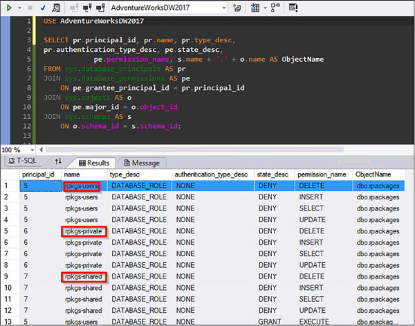
FIGURE 4-71 Query output of added R database roles
After the feature has been enabled, any user with the appropriate permissions can use the CREATE EXTERNAL LIBRARY statement in T-SQL to add packages.
)
)
)
)
)
)
)
)
Install additional R packages
Although the preferred method to install packages is by calling the install.packages() function directly from an R terminal, here you install packages either locally from TSQL using the xp_cmdshell, or from a remote TSQL terminal with the use of the RevoScaleR rxInstallPackages() function. If you are running a SQL Server 2017 instance, package management must be enabled and the queries must be run either with the db_owner or with a user assigned to one of the roles generated before. Similarly, if you have a SQL Server 2016 instance, be sure to run all these scripts either from an elevated window or with the operating system Administrator account.
Install packages from a virtual machine local TSQL query.
Connect to your virtual machine and open SQL Server Management Studio as an Administrator. Before installing packages, you have to enable the xp_cmdshell stored procedure, which enables you to launch command line commands from a TSQL query. In order to do so, execute the following code:
USE MASTER
-- Enable advanced options
EXEC sp_configure 'show advanced options', 1;
GO

RECONFIGURE;
GO

-- Enable xp_cmdshell stored procedure.
EXECUTE SP_CONFIGURE 'xp_cmdshell',1;
GO

RECONFIGURE;
GO
Once the xp_cmdshell stored procedure is enabled, and then execute the following query to call R and pass it to the install.packages() function. As you execute this code, a command line window pops up and the results should be similar to the ones shown in Figure 4-72.
EXEC xp_cmdshell '"C:\Program Files\Microsoft SQL Server\MSSQL14.MSSQLSERVER\R_
SERVICES\bin\R.EXE" cmd -e install.packages(''zoo'')';
GO
)
FIGURE 4-72 Command line window showing the results of installing the package magic
Install packages from a remote TSQL query
Connect to your virtual machine SQL Server instance from your chosen IDE. In order to install packages remotely, you will be using the RevoScaleR rxInstallPackages() function. This function, as most of the RevoScaleR functions, needs to have a specific compute context declared; it functions as the execution target for the function. To create a SQL compute context declaration, you call the RxInSqlServer() function with the connection string to your SQL instance and database as shown in the code below. Then you create a variable containing all the packages that will be installed, and finally you will call the rxInstallPackages() function specifying the compute context and the packages to be installed. Additionally, you can specify the package installation scope; “private” (just accessible by the current user) or “shared” (accessible by all users); and the path to the R Services packages library. If the latter is not specified, R will install the new packages to its default library path.
EXEC sp_execute_external_script
@language =N'R',
@script=N'
sqlcc <- RxInSqlServer(connectionString = "Driver=SQL Server;
                   Server=MSSQLSERVER;
                   Database=AdventureWorksDW2017;
                   UID=sqlvm-admin;
                   PWD=SQVMadmin2017;")
# list of packages to install
pkgs <- c("dplyr")
# Install a package and its dependencies into shared scope
rxInstallPackages(pkgs = pkgs,
verbose = TRUE,
scope = "shared",
computeContext = sqlcc)'
After executing the above code, check that the results are similar to the ones shown in Figure 4-73.
)
FIGURE 4-73 Output of the query containing the rxInstallPackages() function
In order to check that the packages are correctly installed, first query with the following code the location of the packages path. Then follow the path on your virtual machine to check that the directories dplyr and zoo (the packages you have installed in this section) are correctly created.
EXECUTE sp_execute_external_script
    @language = N'R'
   ,@script = N'OutputDataSet <- data.frame(.libPaths());'
WITH RESULT SETS (([DefaultLibraryName] VARCHAR(MAX) NOT NULL));
GO
Finally, whether you installed packages from local or remotely, you can load them into an empty R session to check once again that they are correctly installed and ready to be used in R-TSQL scripts by executing the following code:
   EXEC sp_execute_external_script
@language =N'R',
@script=N'
# load the binaries in dplyr
library(dplyr)'
The output should resemble the one shown in Figure 4-74.
)
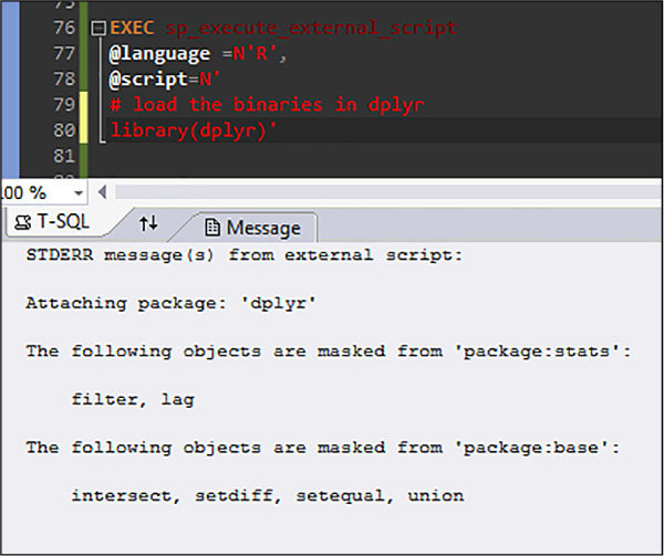
FIGURE 4-74 Results from loading the dplyr package into an empty R session
First steps in SQL Server Machine Learning
The main purpose of Machine Learning Services in SQL Server is providing data engineers and data scientists with an analytical engine capable of performing data science tasks removing the need to move data unnecessarily, or uploading it to external services that might expose your data to security risks. In order to accomplish this, SQL Server Machine Learning executes as a parallel engine with full connectivity to the relational database system, with the ability to run scripts either from SQL Queries or from the R or Python engine, but with minimum data movement from the relational stores to memory stores that R and Python can handle.
Set up SQL Server Machine Learning Services.
Follow the previous set up steps if you have not done so. Most importantly, be sure that the External Scripts Enabled property has a run_value equal to 1, otherwise you will not be able to execute Python or R Scripts.
Develop your R or Python solutions.
Developing R or Python solutions against a development workstation becomes extremely easy with our actual setup. Typically, a data scientist uses R or Python on their own machine to develop a solution with a given set of data. With your actual configuration using an Azure Virtual Machine you are able to connect remotely in order to explore data, build, and tune predictive models and deploy a production quality model to a production scoring scenario directly from your client workstation, without having to move data or ensure that your local scripts will execute on the remote instance. In order to develop your machine learning solutions, you have to:
Choose a development IDE Whether you will work remotely or locally there is a multitude of IDEs from which you could choose in order to develop your solution. The main requirement for your IDE is that it should be able to connect to SQL Server Instances in order to execute R and Python scripts embedded in TSQL Stored procedures. A few of the available options are:
Visual Studio 2017 with the Data Science and Analytical Applications Workload installed.
Visual Studio 2015 with R Tools and Python tools for Visual Studio.
Visual Studio Code with the mssql Extension installed.
SQL Server Management Studio.
Others, such as R Studio, IPython / Jupyter Notebooks, or simple notepad editing with command line execution.
Work remotely or locally The usual walkthrough for a data science solution requires you to copy a table or dataset to your local machine, load it up in memory, and then start from there the data science cycle. However, Machine Learning Services allows you to develop your scripts remotely pushing their execution to the SQL Server instance without having to copy the data to your local environment. This is done through the RevoScaleR and RevoScalePy libraries, which push many of the loading and computing tasks to the server, avoiding costly local executions. In order to work remotely, configure your IDE to connect to your VM and its SQL Server Instance as you have seen before, and all the scripts developed locally will be executed remotely in the development workstation.
Embed R or Python scripts in Transact-SQL stored procedures Once the developed code is fully optimized, wrap it in a stored procedure in order to avoid unnecessary data movement, optimize data processing tasks, and schedule your machine learning or advanced analytics step into a regular ETL or other scheduled tasks.
Optimize processes When the model is ready to scale on enterprise data, the data scientist will often work with the DBA or SQL developer to optimize processes such as:
Feature engineering
Data ingestion and data transformation
Scoring
Traditionally data scientists using R have had problems with both performance and scale, especially when using large dataset. That is because the common runtime implementation is single-threaded and can accommodate only those data sets that fit into the available memory on the local computer. Integration with SQL Server Machine Learning Services provides multiple features for better performance, with more data:
RevoScaleR This R package contains implementations of some of the most popular R functions, redesigned to provide parallelism and scale. The package also includes functions that further boost performance and scale by pushing computations to the SQL Server computer, which typically has far greater memory and computational power.
Revoscalepy This Python library, new and available only in SQL Server 2017 CTP 2.0, implements the most popular functions in RevoScaleR, such as remote compute contexts, and many algorithms that support distributed processing.
Choose the best language for the task. R is best for statistical computations that are difficult to implement using SQL. For set-based operations over data, leverage the power of SQL Server to achieve maximum performance. Use the in-memory database engine for very fast computations over columns.
Deploy and consume
After the R script or model is ready for production use, a database developer might embed the code or model in a stored procedure, deploy a web service, or create predictions based on a stored model with views and/or stored procedures that make use of the TSQL PREDICT clause, so that the saved R or Python code can be called from an application. Storing and running R code from SQL Server has many benefits: you can use the convenient Transact-SQL interface, and all computations take place in the database, avoiding unnecessary data movement.
After deployment, you can integrate predictions and recommendations of your model with further architecture in other apps that are friendlier to the end user. The most common approach is to consult the deployed machine learning solution through PowerBI, and consume its output directly from the application. This allows you to compare quickly predicted data against other queries, cube queries, and historicals while at the same time developing a graphical interface to convey a complete message about your data science problem and the developed solution.
Although PowerBI is one of the most common consumption applications, you are not restricted to it. Once your model has been operationalized by the data engineer, you can consume it from Reporting Services, Analysis Services, Tableau, command line applications, Azure Services, and any other software that can connect to your SQL Server instance and run queries against it.
Execute R and scripts inside T-SQL statements
In this section, you work through a full machine learning development cycle, from exploring the data, creating a model, embedding scripts and functions in T-SQL statements, and then using the model to create predictions and plots.
First steps in embedding R in a T-SQL statement
The following development cycle will be executed from Visual Studio 2017. Visual Studio 2017 should already be configured with the Data Science And Analytical Application and the Data Storage And Processing workloads, as shown in Figure 4-75.
)
FIGURE 4-75 Workloads to enable when installing Visual Studio Code
Open Visual Studio 2017 and under the R Tools menu, click Data Science Settings. A dialog box warns you about changing Visual Studio’s window layout. Accept and proceed to changing the windows to a more development friendly setup.
Open the new project window (CTRL + Shift + N) and create an R Project. Right-click anywhere on the solution explorer pane and add a new existing as shown in Figure 4-76.
)
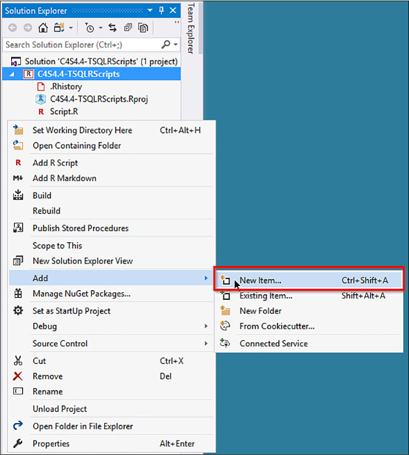
FIGURE 4-76 Add a new SQL Script to your Visual Studio R Project
Select the SQL Query file, and name your file 01_ExecuteBasic_TSQLR.sql. As soon as the SQL editor shows up, copy and paste the following code:
   EXEC sp_execute_external_script
  @language =N'R',
  @script=N'OutputDataSet<-InputDataSet',
  @input_data_1 =N'SELECT 1 AS hello'
  WITH RESULT SETS (([hello] int not null));
GO
In order to execute the code, first you must connect to your virtual machine SQL Server instance. If you try to execute the above script by invoking the keyboard shortcut CTRL + SHIFT + E, a Connect window will be displayed as shown in Figure 4-77.
)
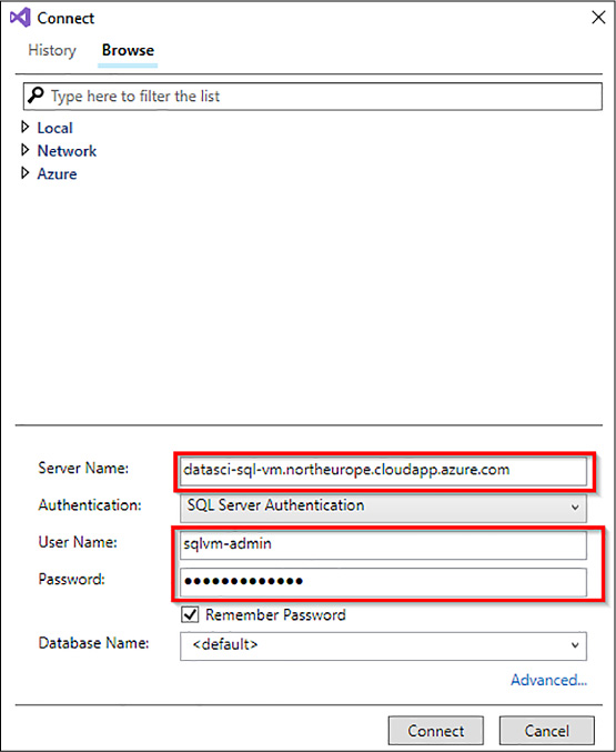
FIGURE 4-77 Connect to your VM SQL Instance from Visual Studio
Fill the fields with your Azure Virtual Machine DNS address, user name, and password, ensuring to select SQL Server Authentication as your Authentication mode. Click Connect.
If your server is configured correctly, you should see the following output.
)
FIGURE 4-78 Correct output from TSQL R script
If you get any errors from this query, installation might be incomplete. After adding the feature using the SQL Server Setup Wizard, you must take some additional steps to enable use of external code libraries. Refer to the section Configure SQL Server To Allow The Execution of R Script in Skill 4.4.
Make sure that the Launchpad service is running. Depending on your environment, you might need to enable the R worker accounts to connect to SQL Server, install additional network libraries, enable remote code execution, or restart the instance after everything is configured.
Working with inputs and outputs
In order to work with R code in SQL Server, you have two options:
Wrap the R script with the sp_execute_external_script system stored procedure, or
Make a call to a stored model using the PREDICT clause of SQL Server 2017.
In the following development, you will be using the stored procedure method in order to execute R code from TSQL queries. The stored procedure is needed for starting the R runtime within the SQL Server context, passing data to the R engine, managing R sessions securely, and returning any output to the client connecting to SQL Server.
A first approach to handle R within TSQL is to create a dummy table, query it using TSQL and R within a stored procedure, and make sure the output is the same. First, run the following code in your Visual Studio 2017 SQL script editor to create a test table.
CREATE TABLE RTestData ([Pi] int not null) ON [PRIMARY]
INSERT INTO RTestData   VALUES (3);
INSERT INTO RTestData   VALUES (14);
INSERT INTO RTestData   VALUES (159) ;
GO
After creating the test table, query the table using first a traditional Select TSQL statement.
SELECT * FROM RTestData
Instead of querying the table with a regular TSQL query, now you query the table using an R script. The following code first executes the traditional TSQL query and saves the results as the variable InputDataSet in the R session, and then the value is saved to the output variable and returned as a result set to the client executing the stored procedure. The language must be defined as R and the script will always be defined as a string within the @script variable.
EXECUTE sp_execute_external_script
      @language = N'R'
    , @script = N' OutputDataSet <- InputDataSet;'
    , @input_data_1 = N' SELECT *  FROM RTestData;'
    WITH RESULT SETS (([NewColName] int NOT NULL));
Both outputs returned to Visual Studio 2017 should be the same. The WITH RESULT SETS clause defines the schema of the returned data table for SQL Server.
Changing the default input and output variable names can be done by declaring the @input_data_1_name and @output_data_1_name variables, as shown in the next script.
EXECUTE sp_execute_external_script
  @language = N'R'
  , @script = N' SQL_Out <- SQL_In;'
  , @input_data_1 = N' SELECT 12 as Col;'
  , @input_data_1_name  = N'SQL_In'
  , @output_data_1_name =  N'SQL_Out'
  WITH RESULT SETS (([NewColName] int NOT NULL));
Be careful when writing your R script, because unlike TSQL, R is case sensitive and will differentiate names based on their case. In all cases, variable names must follow the rules for valid SQL statements. Before declaring @input_data_1_name and @output_data_1_name, you must always declare @input_data_1 and @output_data_1 first.
You can also generate data from within an R script and output it to SQL Server and the client used. This is done by using a valid TSQL statement as @input_data_1, but then developing a script that does not use this input, as shown in the code below:
EXECUTE sp_execute_external_script
    @language = N'R'
   , @script = N' mytextvariable <- c("hello", " ", "world");
       OutputDataSet <- as.data.frame(mytextvariable);'
   , @input_data_1 = N' SELECT 1 as Temp1'
   WITH RESULT SETS (([Col1] char(20) NOT NULL));
R and SQL data types and data objects
Given that you have to match schemas and data types when in- and out-putting data into an R script, there are a few common issues that usually arise. These are:
Data types sometimes do not match.
Implicit conversions might take place.
Cast and convert operations are sometimes required.
R and SQL use different data objects.
Becuse R returns its resulting data to SQL Server, it must always return it as a data.frame object. Any other object used within the R script, whether it be lists, variables, vectors, matrices, or factors, must be encapsulated in a data.frame in order to be passed to SQL Server. Even a trained binary model must be encapsulated and transformed to a data.frame in order to store it in SQL Server. You work through a couple of these transformations in the next code examples.
Take a look at the following two “Hello World” scripts in R. The first stores a string array in a temporary variable and later is transformed to a data.frame object. The second script directly defines a data.frame within the output variable.
EXECUTE sp_execute_external_script
       @language = N'R'
     , @script = N' mytextvariable <- c("hello", " ", "world");
       OutputDataSet <- as.data.frame(mytextvariable);'
     , @input_data_1 = N' ';

EXECUTE sp_execute_external_script
        @language = N'R'
      , @script = N' OutputDataSet<- data.frame(c("hello"), " ", c("world"));'
      , @input_data_1 = N'  '
The results of these examples can be seen in Figures 4-79 and Figures 4-80 below. As you execute both examples, you will soon find that the output is completely different. Example 1 outputs a vector with one column and three rows, whereas example 2 outputs a vector with three columns and only one value in each. Without going into details, the reason for this behavior lies in that R implements ‘column-major’ order in accessing matrices and data.frames. If you attach the structure function, str(), to any of the scripts you will get additional information as to the nature of each of the R objects. To view the output of the str() functions, or any other R functions that return messages and outputs to the command line, switch to the Messages pane/tab in VS Code, Visual Studio 2017, or SQL Server Management Studio. The following code exemplifies this behavior.
EXECUTE sp_execute_external_script
  @language = N'R',
  @script = N' OutputDataSet <- data.frame(c("hello"), " ", c("world"));
    str(OutputDataSet)' ,
  @input_data_1 = N'  ';
You can inspect the str() output for both examples in Figure 4-79 and Figure 4-80.
)
FIGURE 4-79 str() output from defining a data.frame directly from an array
)
FIGURE 4-80 str() output from an R array
R and SQL Server do not use the same data types, therefore when you run a query in SQL Server to get data and then pass that to the R runtime, some type of implicit conversion usually takes place. Another set of conversions takes place when you return data from R to SQL Server. SQL Server pushes the data from the input query to the R process managed by the Launchpad service and converts it to an internal representation for greater efficiency. The R runtime loads the data into a data.frame object and performs the script operations on the data. The R engine then returns the data to SQL Server using a secured internal connection and presents the data in terms of SQL Server data types.
As an example of this engine’s mechanics, you can run the following code and examine its output both from SQL and from the R Script implementation. You need to have one of the AdventureWorksDW databases restored.
EXECUTE sp_execute_external_script
        @language = N'R',
        @script = N' str(InputDataSet);
        OutputDataSet <- InputDataSet;',
        @input_data_1 = N'
            SELECT ReportingDate
                , CAST(ModelRegion as varchar(50)) as ProductSeries
                , Amount
            FROM [AdventureWorksDW2017].[dbo].[vTimeSeries]
            WHERE [ModelRegion] = ''M200 Europe''
            ORDER BY ReportingDate ASC ;'
WITH RESULT SETS undefined;
The results are shown in Figure 4-81.
)
FIGURE 4-81 Data types conversion from SQL table to an R data.frame
You can see that the data has been converted from a datetime column into a POSIXct R time data type. The column “ProductSeries,” on the other hand, is specified as a factor column; this is a common R transformation on character columns, typical of categorical variables, to a numeric column with a string look up (Factors). Finally, the ‘Amount’ column has been stored correctly as a numeric column.
In order to avoid any problems when handling data to the R engine or acquiring data from an R script, be sure to follow the following steps to avoid errors:
Test your data in advance and verify columns or values in your schema that could be a problem when passed to R code.
Specify columns in your input data source individually, rather than using SELECT *, and know how each column will be handled.
Perform explicit casts as necessary when preparing your input data, to avoid undesired casts and/or conversions of your data types.
Avoid passing columns of data (such as GUIDS or rowguids) that cause errors and are not useful for modeling.
Applying R functions on SQL Server data
Up to this point, you have successfully executed basic R scripts remotely on an Azure SQL Server Virtual Machine within a TSQL stored procedure. Now you can start using the full power of R to leverage many statistical and complex analysis tasks that, if you tried to implement in TSQL, would take many lines of code, as compared to just a few lines in R.
As an example, you first use a function from the internally installed package, stats, to generate an array of normally distributed number given a mean and a standard deviation. The function to generate random normally distributed numbers is called rnorm() and can be called on an R command line like the following:
rnorm(<number of samples>, mean = <desired mean>, sd = <desired std deviation>)
To call this function from TSQL, encapsulate it in the sp_execute_external_script as you have already done:
EXEC sp_execute_external_script
        @language = N'R',
        @script = N'
            OutputDataSet <- as.data.frame(rnorm(100, mean = 50, sd =3));',
        @input_data_1 = N'   ;'
WITH RESULT SETS (([Density] float NOT NULL));
In this case, the number of samples, mean and standard deviation are hard coded into the call. If you would like to have different inputs directly from TSQL, you need to define those parameters as variables and pass them to the sp_execute_external_script stored procedure, as shown:
CREATE PROCEDURE MyRNorm (@param1 int, @param2 int, @param3 int)
AS
    EXEC sp_execute_external_script
      @language = N'R'
    , @script = N'
         OutputDataSet <- as.data.frame(rnorm(mynumbers, mymean, mysd));'
    , @input_data_1 = N'   ;'
    , @params = N' @mynumbers int, @mymean int, @mysd int'
    , @mynumbers = @param1
    , @mymean = @param2
    , @mysd = @param3
    WITH RESULT SETS (([Density] float NOT NULL));
The stored procedure call defines additional parameters that are passed to the R function in the R services. The line beginning with @params defines all variables used by the R code, and the corresponding SQL data types, and the following lines define which TSQL parameters map to which R variables. In order to execute this function call, just copy and execute the following line of code:
EXEC MyRNorm @param1 = 100,@param2 = 50, @param3 = 3
Create a predictive model
One of the most powerful uses of R is as a machine learning engine. Many algorithms have been developed to handle different types of machine learning problems, and many problems and algorithms are still better solved from R than from competing languages, such as Python, Julia, or fully implemented machine learning / deep learning services such as TensorFlow. Although algorithms and packages such as XGBoost, e1701, caret, nnet, or randomforest are widely used, you create a simple regression model in this section and store it to the SQL relational engine. Furthermore, you develop the models with Microsoft R Server functions, which are optimized for parallel and distributed computation.
The model you will be developing is a linear model to predict the duration of the eruption for the Old Faithful geyser in Yellowstone National Park, Wyoming, USA based on the waiting time between eruptions. The data is part of the sample data that comes with the R installation, and further information can be found by typing ?faithful on an R command line (*see Figure 4-82).
)
FIGURE 4-82 R command line and R Help window with faithful dataset information
First, create a table to save the eruptions data.
CREATE TABLE Eruptions ([duration] float not null, [waiting] int not null)
INSERT INTO Eruptions
EXEC sp_execute_external_script
        @language = N'R'
        , @script = N'eruptions <- faithful;'
        , @input_data_1 = N''
        , @output_data_1_name = N'eruptions'
Inspect the data to make sure it has been copied successfully by querying it with a simple SELECT:
SELECT * FROM Eruptions
This script essentially copies the faithful data into a relational table. In order to create the model, you need to define a relationship between the columns of your dataset. Because you have a simple regression, the model is duration ~ waiting, which reads ‘duration is dependent on waiting’. This formula is defined within the R Server rxLinMod() function in the code below:
DROP PROCEDURE IF EXISTS generate_linear_model;
GO
CREATE PROCEDURE generate_linear_model
AS
BEGIN
    EXEC sp_execute_external_script
    @language = N'R'
    , @script = N'lrmodel <- rxLinMod(formula = duration ~ waiting, data =
FaithfulEruptions);
        trained_model <- data.frame(payload = as.raw(serialize(lrmodel,
connection=NULL)));'
    , @input_data_1 = N'SELECT [duration], [waiting] FROM Eruptions'
    , @input_data_1_name = N'FaithfulEruptions'
    , @output_data_1_name = N'trained_model'
    WITH RESULT SETS ((model varbinary(max)));
END;
GO
The output should resemble the one shown in Figure 4-83.
)
FIGURE 4-83 Results of creating the train model stored procedure
After you defined the store procedure that trains the linear model, you need to save it to a table for future use. A trained model is essentially binary data that tells a scoring algorithm how to combine the columns of dataset in order to produce an output. As a simple example think of matrix algebra, and let the situation be described as AX=Y, where X is your input, Y your output, and A your model. A is just a matrix that can be hashed and stored as a single value in a table. Generally speaking, models are much more complex than simple matrices, but for this example the abstraction suffices. Create the table running the following code:
CREATE TABLE faithful_eruptions_models (
    model_name varchar(30) not null default('default model') primary key,
    model varbinary(max) not null);
Finally, you can populate the model table by executing the training stored procedure, and returning the output to the models table, as shown below in Figure 4-84.
INSERT INTO faithful_eruptions_models (model)
EXEC generate_linear_model;
Unfortunately, this table will not allow you to stored successive trained models because the table has no ID column, and the model is constantly being saved with the same name in its ‘model_name’ column. In order to sort this problem, you can change the naming scheme to something more descriptive, run the training stored procedure one more time, and query the models table to see the results.
UPDATE faithful_eruptions_models
SET model_name = 'rxLinMod ' + format(getdate(), 'yyyy.MM.HH.mm', 'en-gb')
WHERE model_name = 'default model'
GO

INSERT INTO faithful_eruptions_models (model)
EXEC generate_linear_model;
GO

SELECT * FROM faithful_eruptions_models
You will be able to see that the models are stored as a hex value under the ‘model’ column, as shown in Figure 4-84.
)
FIGURE 4-84 Stored serialized linear models in a SQL table
In general, remember these when working with SQL parameters and R variables in TSQL:
All SQL parameters mapped to R script must be listed by name in the @params argument.
To output one of these parameters, add the OUTPUT keyword in the @params list.
After listing the mapped parameters, provide the mapping, line by line, of SQL parameters to R variables, immediately after the @params list.
Predict and plot from model
Scoring based on the stored models is easily done by recalling the model from the table, applying the model on a new set of data, and storing the output in a table. Scoring is also known as predicting, estimating, or generating an output from a trained model based on the data on which the output or prediction is desired.
The Old Faithful data registers waiting times from 43 minutes up to 96 minutes. However, what would be the expected duration of an eruption if you went to Yellowstone and had to wait 120 minutes? Apart from your disillusion that Old Faithful is making truer its old state more that its faithful, you could quickly pull out your linear model and give some hope to the people at the area by telling them that longer waits only bring more spectacular eruptions. In order to do so, you must provide the additional waiting times to make a prediction of how long the geyser will erupt. Create a new table with the new waiting times with the following code:
CREATE TABLE [dbo].[NewEruptions](
        [duration] float null,
        [waiting] int not null) ON [PRIMARY]
GO

INSERT [dbo].[NewEruptions] ([waiting])
VALUES (20),  (25),  (30), (35), (40), (100), (105), (110), (115), (120)
At this point your models’ table must have several different models, all trained on different data, or at different times, or with different parameters. To get predictions based on one specific model, you must write a SQL script that does the following:
Gets the model you want.
Gets the new input data.
Calls an R prediction function that is compatible with that model.
Given that you have generated a model using Microsoft Machine Learning Server functions, you will also generate the scoring / prediction using the rxPredict() function, instead of the generic R predict() function. You do this with the following code:
DECLARE @eruptionsmodel varbinary(max) = (SELECT model FROM [dbo].[faithful_eruptions_
models] WHERE model_name = 'default model');
EXEC sp_execute_external_script
    @language = N'R'
    , @script = N'
            current_model <- unserialize(as.raw(eruptionsmodel));
            new <- data.frame(ExpectedEruptions);
            predicted.duration <- rxPredict(current_model, new);
            str(predicted.duration);
            OutputDataSet <- cbind(new, predicted.duration);
            '
    , @input_data_1 = N' SELECT waiting FROM [dbo].[NewEruptions] '
    , @input_data_1_name = N'ExpectedEruptions'
    , @params = N'@eruptionsmodel varbinary(max)'
    , @eruptionsmodel = @eruptionsmodel
WITH RESULT SETS (([expected_waiting] INT, [predicted_duration] FLOAT))
The initial select statement selects a model from the model table. Once the model is in memory, it is unserialized (converted from a hex binary to a usable R object) and stored as an R variable. Then, applying the predict formula on the new data, and using the stored model, a new set of predicted durations is generated. The str() function is added in order to check that the output dataset matches in schema and data type with the WITH RESULT SET clause. The results of the prediction can be seen in Figure 4-85.
)
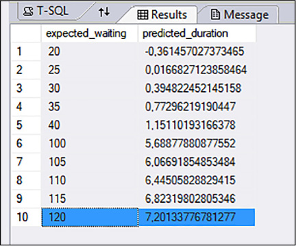
FIGURE 4-85 Old Faithful predicted eruption durations from estimated waiting times
In the case of a two hour waiting time you will be delighted to have an eruption of little over seven minutes.
An important additional parameter is the @parallel=1 flag. In this example your data is rather small, but suppose you have a large dataset with millions of rows and thousands of columns, you will probably need to optimize speeds by computing in parallel as much as you can. The @parallel flag enables parallel execution for your R script. Parallel execution generally provides benefits only when working with very large data. The SQL database engine might decide that parallel execution is not needed. Moreover, the SQL query that gets your data must be capable of generating a parallel query plan. When using the option for parallel execution, you must specify the output results schema in advance, by using the WITH RESULT SETS clause. Specifying the output schema in advance allows SQL Server to aggregate the results of multiple parallel datasets, which otherwise might have unknown schemas. This parameter often does not have any effect when training a model; it is mostly used when scoring a data set. If you wish to train complex algorithms with large training data, it is recommended that you use Microsoft R Server functions and libraries. The functions and algorithms in these services are specially engineered to train on parallel and distributed data.
Finally, you create a plot of the data and the trained model. Many clients, such as SQL Server Management Studio, cannot display plots created using an R script. Visual Studio and VS Code can display R plots, but these plots are displayed directly from the local memory and a local R session running as a command line window. In your current setup, the process to generate R plots is to create the plot within your R script, write the image to a file, or serialize it and save it in a table and then open the image file or render the serialized table image.
The following example demonstrates how to create a simple graphic using a plotting function included by default with R. The image is saved to the specified file, and it is returned as a serialized SQL value by the stored procedure.
EXECUTE sp_execute_external_script
 @language = N'R'
 , @script = N'
     imageDir <- ''C:\\Users\\Public'';
     image_filename = tempfile(pattern = "plot_", tmpdir = imageDir, fileext =
".jpg")
     print(image_filename);
     jpeg(filename=image_filename,  width=600, height = 800);
     print(plot(duration~waiting, data=InputDataSet, xlab="Waiting (mins)",
 ylab="Eruption Duration(mins)", main = "Old Faithful Geyser Eruptions"));
     abline(lm(duration~waiting, data = InputDataSet));
     dev.off();
     OutputDataSet <- data.frame(data=readBin(file(image_filename, "rb"),
what=raw(), n=1e6));
     '
  , @input_data_1 = N'SELECT duration, waiting from [dbo].[Eruptions]'
  WITH RESULT SETS ((plot varbinary(max)));
When executing the code above be sure to go to the C:\User\Public directory to retrieve the image file. The method for creating a plot and saving it to an image essentially is opening a print device, plotting to it, adding the abline, and then closing the device. The resulting plot can be seen in Figure 4-86. From the graph you can quickly identify two trends in the eruptions data:
)
There are two clusters of eruptions: short and frequent and long and less frequent.
There is a linear correlation between waiting time and eruption time, thus the modeling method you have used is valid in this situation.
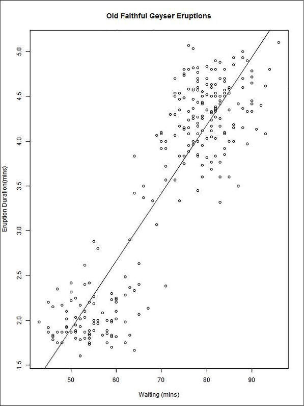
FIGURE 4-86 Old Faithful plot of waiting minutes vs. eruption minutes, with a linear fit of the points