How to Change the Appearance of a Workbook in Microsoft Excel 2016

Change the appearance of data based on its value

Recording information such as package volumes, vehicle miles, and other business data in a worksheet enables you to make important decisions about your operations. And as you saw earlier in this chapter, you can change the appearance of data labels and the worksheet itself to make interpreting your data easier.

Another way you can make your data easier to interpret is to have Excel change the appearance of your data based on its value. The formats that make this possible are called conditional formats, because the data must meet certain conditions, defined in conditional formatting rules, to have a format applied to it. In Excel, you can define conditional formats that change how the app displays data in cells that contain values above or below the average values of the related cells, that contain values near the top or bottom of the value range, or that contain values duplicated elsewhere in the selected range.

When you select which kind of condition to create, Excel displays a dialog box that contains fields and controls you can use to define your rule. If your cells already have conditional formats applied to them, you can display those formats.

Click to view larger image

Manage conditional formats by using the Conditional Formatting Rules Manager

You can control your conditional formats in the following ways:

• Create a new rule.
• Change a rule.
• Remove a rule.
• Move a rule up or down in the order.
• Control whether Excel continues evaluating conditional formats after it finds a rule to apply.
• Save any rule changes and stop editing rules.
• Save any rule changes and continue editing.
• Discard any unsaved changes.

Clicking the New Rule button in the Conditional Formatting Rules Manager opens the New Formatting Rule dialog box. The commands in the New Formatting Rule dialog box duplicate the options displayed when you click the Conditional Formatting button in the Styles group on the Home tab. You can use those controls to define your new rule and the format to be displayed if the rule is true.

Create rules by using the New Formatting Rule dialog box

Important

Excel doesn’t check to make sure that your conditions are logically consistent, so you need to be sure that you plan and enter your conditions correctly.

You can also create three other types of conditional formats in Excel: data bars, color scales, and icon sets. Data bars summarize the relative magnitude of values in a cell range by extending a band of color across the cell.

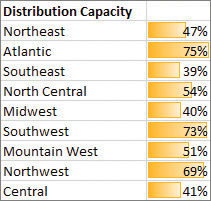
Apply data bars to view how values compare to one another

You can create two types of data bars in Excel 2016: solid fill and gradient fill. When data bars were introduced in Excel 2007, they filled cells with a color band that decreased in intensity as it moved across the cell. This gradient fill pattern made it a bit difficult to determine the relative length of two data bars because the end points weren’t as distinct as they would have been if the bars were a solid color. In Excel 2016 you can choose between a solid fill pattern, which makes the right edge of the bars easier to discern, and a gradient fill, which you can use if you share your workbook with colleagues who use Excel 2007.

Excel 2016 also draws data bars differently than in Excel 2007. Excel 2007 drew a very short data bar for the lowest value in a range and a very long data bar for the highest value. The problem was that similar values could be represented by data bars of very different lengths if there wasn’t much variance among the values in the conditionally formatted range. In Excel 2016, data bars compare values based on their distance from zero, so similar values are summarized by using data bars of similar lengths.

TIP

Excel 2016 data bars summarize negative values by using bars that extend to the left of a baseline that the app draws in a cell.

Color scales compare the relative magnitude of values in a cell range by applying colors from a two-color or three-color set to your cells. The intensity of a cell’s color reflects the value’s tendency toward the top or bottom of the values in the range.

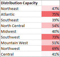
Apply a color scale to emphasize the magnitude of values within a cell range

Icon sets are collections of three, four, or five images that Excel displays when certain rules are met.

Icon sets show how values compare to a standard

When icon sets were introduced in Excel 2007, you could apply an icon set as a whole, but you couldn’t create custom icon sets or choose to have Excel 2007 display no icon if the value in a cell met a criterion. In Excel 2016, you can display any icon from any set for any criterion or display no icon, plus you can edit your format in other ways so it summarizes your data exactly as you want it to.

When you click a color scale or icon set in the Conditional Formatting Rules Manager and then click the Edit Rule button, you can control when Excel applies a color or icon to your data.

Important

Be sure to not include cells that contain summary formulas in your conditionally formatted ranges. The values, which could be much higher or lower than your regular cell data, could throw off your comparisons.

To create a conditional formatting rule

1. Select the cells you want to format.
2. On the Home tab, in the Styles group, click the Conditional Formatting button, point to Highlight Cells Rules, and then click the type of rule you want to create.
3. In the rule dialog box that appears, set the rules for the condition.
4. Click the arrow next to the with box, and then click Custom Format.
5. Use the controls in the Format Cells dialog box to define the custom format.
6. Click OK to close the Format Cells dialog box.
7. Click OK to close the rule dialog box.

To edit a conditional formatting rule

1. Select the cells to which the rule is applied.
2. Click the Conditional Formatting button, and then click Manage Rules.
3. In the Conditional Formatting Rules Manager, click the rule you want to edit.
4. Click Edit Rule.
5. Use the controls in the Edit Formatting Rule dialog box to change the rule settings.
6. Click OK twice to close the Edit Formatting Rule dialog box and the Conditional Formatting Rules Manager.

To change the order of conditional formatting rules

1. Select the cells to which the rules are applied.
2. Click the Conditional Formatting button, and then click Manage Rules.
3. In the Conditional Formatting Rules Manager, click the rule you want to move.

4. Click the Move Up button to move the rule up in the order.

   Or

   Click the Move Down button to move the rule down in the order.

5. Click OK.

To stop applying conditional formatting rules when a condition is met

1. Select the cells to which the rule is applied.
2. Click the Conditional Formatting button, and then click Manage Rules.

3. In the Conditional Formatting Rules Manager, select the Stop If True check box next to the rule where you want Excel to stop.

   

   Click to view larger image

   Stop checking conditional formats if a specific condition is met

4. Click OK.

To create a data bar conditional format

1. Click the Conditional Formatting button, point to Data Bars, and then click the format you want to apply.

To create a color scale conditional format

1. Click the Conditional Formatting button, point to Color Scales, and then click the color scale you want to apply.

To create an icon set conditional format

1. Click the Conditional Formatting button, point to Icon Sets, and then click the icon set you want to apply.

To delete a conditional format

1. Select the cells to which the rules are applied.
2. Click the Conditional Formatting button, and then click Manage Rules.

3. In the Conditional Formatting Rules Manager, click the rule you want to delete.

   

   Click to view larger image

   Delete a conditional format you no longer need

4. Click Delete Rule.
5. Click OK.

To delete all conditional formats from a worksheet

1. Click the Conditional Formatting button, point to Clear Rules, and then click Clear Rules from Entire Sheet.