How to Change the Appearance of a Workbook in Microsoft Excel 2016
- By Curtis Frye
- 10/16/2015
Entering data into a workbook efficiently saves you time, but you must also ensure that your data is easy to read. Microsoft Excel 2016 gives you a wide variety of ways to make your data easier to understand; for example, you can change the font, character size, or color used to present a cell’s contents. Changing how data appears on a worksheet helps set the contents of a cell apart from the contents of surrounding cells. To save time, you can define a number of custom formats and then apply them quickly to the cells you want to emphasize.
You might also want to specially format a cell’s contents to reflect the value in that cell. For example, you could create a worksheet that displays the percentage of improperly delivered packages from each regional distribution center. If that percentage exceeds a threshold, Excel could display a red traffic light icon, indicating that the center’s performance is out of tolerance and requires attention.
This chapter guides you through procedures related to changing the appearance of data, applying existing formats to data, making numbers easier to read, changing data’s appearance based on its value, and adding images to worksheets.
Format cells
Excel worksheets can hold and process lots of data, but when you manage numerous worksheets, it can be hard to remember from a worksheet’s title exactly what data is kept in that worksheet. Data labels give you and your colleagues information about data in a worksheet, but it’s important to format the labels so that they stand out visually. To make your data labels or any other data stand out, you can change the format of the cells that hold your data.
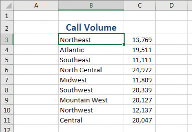
Use formatting to set labels apart from worksheet data
TIP

Deleting a cell’s contents doesn’t delete the cell’s formatting. To delete a selected cell’s formatting, on the Home tab, in the Editing group, click the Clear button (which looks like an eraser), and then click Clear Formats. Clicking Clear All from the same list will remove the cell’s contents and formatting.
Many of the formatting-related buttons on the ribbon have arrows at their right edges. Clicking the arrow displays a list of options for that button, such as the fonts available on your system or the colors you can assign to a cell.
TIP
Clicking the body of the Border, Fill Color, or Font Color button applies the most recently applied formatting to the currently selected cells.
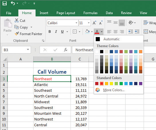
Change font color to help labels and values stand out
You can also make a cell stand apart from its neighbors by adding a border around the cell or changing the color or shading of the cell’s interior.
Add borders to set cells apart from their neighbors
TIP
You can display the most commonly used formatting controls by right-clicking a selected range. When you do, a mini toolbar containing a subset of the Home tab formatting tools appears above the shortcut menu.
If you want to change the attributes of every cell in a row or column, you can click the header of the row or column you want to modify and then select the format you want.
One task you can’t perform by using the tools on the ribbon is to change the default font for a workbook, which is used in the formula bar. The default font when you install Excel is Calibri, a simple font that is easy to read on a computer screen and on the printed page. If you’d prefer to change the default font, you can do so, but only from the Excel Options dialog box, not from the ribbon.
Important

The new standard font doesn’t take effect until you exit Excel and restart the app.
To change the font used to display cell contents
- Select the cell or cells you want to format.
- On the Home tab of the ribbon, in the Font group, click the Font arrow.
- In the font list, click the font you want to apply.
To change the size of characters in a cell or cells
- Select the cell or cells you want to format.
- Click the Font Size arrow.
- In the list of sizes, click the size you want to apply.
To change the size of characters in a cell or cells by one increment
- Select the cell or cells you want to format.
Click the Increase Font Size button.
Or
Click the Decrease Font Size button.
To change the color of a font
- Select the cell or cells you want to format.
- Click the Font Color arrow (not the button).
Click the color you want to apply.
Or
Click More Colors, select the color you want from the Colors dialog box, and then click OK.
To change the background color of a cell or cells
- Select the cell or cells you want to format.
Click the Fill Color arrow (not the button).
Click the color you want to apply.
Or
Click More Colors, select the color you want from the Colors dialog box, and click OK.
)
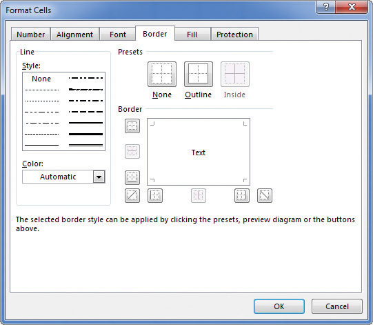
To add a border to a cell or cells
- Select the cell or cells you want to format.
- Click the Border arrow (not the button).
Click the border pattern you want to apply.
Or
Click More Borders, select the borders you want from the Border tab of the Format Cells dialog box, and click OK.
To change font appearance by using the controls on the Font tab of the Format Cells dialog box
- Click the Font dialog box launcher.
- Make the formatting changes you want, and then click OK.
To copy formatting between cells
- Select the cell that contains the formatting you want to copy.
- Click the Format Painter button.
- Select the cells to which you want to apply the formatting.
Or
- Select the cell that contains the formatting you want to copy.
- Double-click the Format Painter button.
- Select cells or groups of cells to which you want to apply the formatting.
- Press the Esc key to turn off the Format Painter.
To delete cell formatting
- Select the cell or cells from which you want to remove formatting.
In the Editing group, click the Clear button.
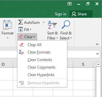
Use the Clear button to delete formats from a cell
- In the menu that appears, click Clear Formats.
To change the default font of a workbook
- Display the Backstage view, and then click Options.
- On the General page of the Excel Options dialog box, in the Use this as the default font list, click the font you want to use.
- In the Font size list, click the font size you want.
- Click OK.
- Exit and restart Excel to complete the default font change.