How to Change the Appearance of a Workbook in Microsoft Excel 2016

Make numbers easier to read

Changing the format of the cells in your worksheet can make your data much easier to read, both by setting data labels apart from the actual data and by adding borders to define the boundaries between labels and data even more clearly. Of course, using formatting options to change the font and appearance of a cell’s contents doesn’t help with idiosyncratic data types such as dates, phone numbers, or currency values.

As an example, consider US phone numbers. These numbers are 10 digits long and have a 3-digit area code, a 3-digit exchange, and a 4-digit line number written in the form (###) ###-####. Although it’s certainly possible to enter a phone number with the expected formatting in a cell, it’s much simpler to enter a sequence of 10 digits and have Excel change the data’s appearance.

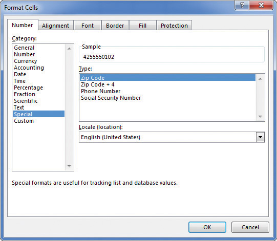
Select built-in number formats from the Special category

You can watch this format in operation if you compare the contents of the active cell and the contents of the formula box for a cell with the Phone Number formatting.

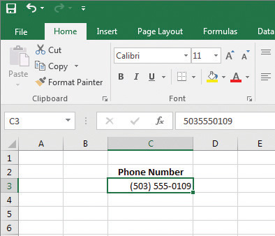
Change the appearance of data without affecting the underlying data

Important

If you enter a 9-digit number in a field that expects a phone number, you won’t get an error message; instead, you’ll get a 2-digit area code. For example, the number 425550012 would be displayed as (42) 555-0012. An 11-digit number would be displayed with a 4-digit area code. If the phone number doesn’t look right, you probably left out a digit or included an extra one, so you should make sure your entry is correct.

Just as you can instruct Excel to expect a phone number in a cell, you can also have it expect a date or a currency amount. You can pick from a wide variety of date, currency, and other formats to best reflect your worksheet’s contents, your company standards, and how you and your colleagues expect the data to appear.

TIP

In the Excel user interface you can make the most common format changes by displaying the Home tab and then, in the Number group, either clicking a button representing a built-in format or selecting a format from the Number Format list.

You can also create a custom numeric format to add a word or phrase to a number in a cell. For example, you can add the phrase per month to a cell with a formula that calculates average monthly sales for a year, to ensure that you and your colleagues will recognize the figure as a monthly average. If one of the built-in formats is close to the custom format you’d like to create, you can base your custom format on the one already included in Excel.

Important

You need to enclose any text to be displayed as part of the format in quotation marks so that Excel recognizes the text as a string to be displayed in the cell.

To apply a special number format

1. Select the cells to which you want to apply the format.
2. On the Home tab, in the Number group, click the Number Format arrow, and then click More Number Formats.
3. In the Format Cells dialog box, in the Category list, click Special.
4. In the Type list, click the format you want to apply.
5. Click OK.

To create a custom number format

1. On the Number Format menu, click More Number Formats.
2. In the Format Cells dialog box, in the Category list, click Custom.
3. Click the format you want to use as the base for your new format.
4. Edit the format in the Type box.
5. Click OK.

To add text to a number format

1. On the Number Format menu, click More Number Formats.
2. In the Format Cells dialog box, in the Category list, click Custom.
3. Click the format you want to use as the base for your new format.

4. In the Type box, after the format, enter the text you want to add, in quotation marks—for example, “boxes”.

   

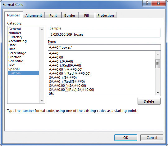
   Define custom number formats that display text after values

5. Click OK.