Introducing DAX

Using common DAX functions

Now that you have seen the fundamentals of DAX and how to handle error conditions, what follows is a brief tour through the most commonly used functions and expressions of DAX.

Aggregation functions

In the previous sections, we described the basic aggregators like SUM, AVERAGE, MIN, and MAX. You learned that SUM and AVERAGE, for example, work only on numeric columns.

DAX also offers an alternative syntax for aggregation functions inherited from Excel, which adds the suffix A to the name of the function, just to get the same name and behavior as Excel. However, these functions are useful only for columns containing Boolean values because TRUE is evaluated as 1 and FALSE as 0. Text columns are always considered 0. Therefore, no matter what is in the content of a column, if one uses MAXA on a text column, the result will always be a 0. Moreover, DAX never considers empty cells when it performs the aggregation. Although these functions can be used on nonnumeric columns without retuning an error, their results are not useful because there is no automatic conversion to numbers for text columns. These functions are named AVERAGEA, COUNTA, MINA, and MAXA. We suggest that you do not use these functions, whose behavior will be kept unchanged in the future because of compatibility with existing code that might rely on current behavior.

The functions you learned earlier are useful to perform the aggregation of values. Sometimes, you might not be interested in aggregating values but only in counting them. DAX offers a set of functions that are useful to count rows or values:

• COUNT operates on any data type, apart from Boolean.

• COUNTA operates on any type of column.

• COUNTBLANK returns the number of empty cells (blanks or empty strings) in a column.

• COUNTROWS returns the number of rows in a table.

• DISTINCTCOUNT returns the number of distinct values of a column, blank value included if present.

• DISTINCTCOUNTNOBLANK returns the number of distinct values of a column, no blank value included.

COUNT and COUNTA are nearly identical functions in DAX. They return the number of values of the column that are not empty, regardless of their data type. They are inherited from Excel, where COUNTA accepts any data type including strings, whereas COUNT accepts only numeric columns. If we want to count all the values in a column that contain an empty value, you can use the COUNTBLANK function. Both blanks and empty values are considered empty values by COUNTBLANK. Finally, if we want to count the number of rows of a table, you can use the COUNTROWS function. Beware that COUNTROWS requires a table as a parameter, not a column.

The last two functions, DISTINCTCOUNT and DISTINCTCOUNTNOBLANK, are useful because they do exactly what their names suggest: count the distinct values of a column, which it takes as its only parameter. DISTINCTCOUNT counts the BLANK value as one of the possible values, whereas DISTINCTCOUNTNOBLANK ignores the BLANK value.

Logical functions

Sometimes we want to build a logical condition in an expression—for example, to implement different calculations depending on the value of a column or to intercept an error condition. In these cases, we can use one of the logical functions in DAX. The earlier section titled “Handling errors in DAX expressions” described the two most important functions of this group: IF and IFERROR. We described the IF function in the “Conditional statements” section, earlier in this chapter.

Logical functions are very simple and do what their names suggest. They are AND, FALSE, IF, IFERROR, NOT, TRUE, and OR. For example, if we want to compute the amount as quantity multiplied by price only when the Price column contains a numeric value, we can use the following pattern:

Sales[Amount] = IFERROR ( Sales[Quantity] * Sales[Price], BLANK ( ) )

If we did not use IFERROR and if the Price column contained an invalid number, the result for the calculated column would be an error because if a single row generates a calculation error, the error propagates to the whole column. The use of IFERROR, however, intercepts the error and replaces it with a blank value.

Another interesting function in this category is SWITCH, which is useful when we have a column containing a low number of distinct values, and we want to get different behaviors depending on its value. For example, the column Size in the Product table contains S, M, L, XL, and we might want to decode this value in a more explicit column. We can obtain the result by using nested IF calls:

'Product'[SizeDesc] =
IF (
    'Product'[Size] = "S",
    "Small",
    IF (
        'Product'[Size] = "M",
        "Medium",
        IF (
            'Product'[Size] = "L",
            "Large",
            IF (
                'Product'[Size] = "XL",
                "Extra Large",
                "Other"
            )
        )
    )
)

A more convenient way to express the same formula, using SWITCH, is like this:

'Product'[SizeDesc] =
SWITCH (
    'Product'[Size],
    "S", "Small",
    "M", "Medium",
    "L", "Large",
    "XL", "Extra Large",
    "Other"
)

The code in this latter expression is more readable, though not faster, because internally DAX translates SWITCH statements into a set of nested IF functions.

SWITCH (
   TRUE (),
   Product[Size] = "XL" && Product[Color] = "Red", "Red and XL",
   Product[Size] = "XL" && Product[Color] = "Blue", "Blue and XL",
   Product[Size] = "L" && Product[Color] = "Green", "Green and L"
)

Information functions

Whenever there is the need to analyze the type of an expression, you can use one of the information functions. All these functions return a Boolean value and can be used in any logical expression. They are ISBLANK, ISERROR, ISLOGICAL, ISNONTEXT, ISNUMBER, and ISTEXT.

It is important to note that when a column is passed as a parameter instead of an expression, the functions ISNUMBER, ISTEXT, and ISNONTEXT always return TRUE or FALSE depending on the data type of the column and on the empty condition of each cell. This makes these functions nearly useless in DAX; they have been inherited from Excel in the first DAX version.

You might be wondering whether you can use ISNUMBER with a text column just to check whether a conversion to a number is possible. Unfortunately, this approach is not possible. If you want to test whether a text value is convertible to a number, you must try the conversion and handle the error if it fails. For example, to test whether the column Price (which is of type string) contains a valid number, one must write

Sales[IsPriceCorrect] = NOT ISERROR ( VALUE ( Sales[Price] ) )

DAX tries to convert from a string value to a number. If it succeeds, it returns TRUE (because ISERROR returns FALSE); otherwise, it returns FALSE (because ISERROR returns TRUE). For example, the conversion fails if some of the rows have an “N/A” string value for price.

However, if we try to use ISNUMBER, as in the following expression, we always receive FALSE as a result:

Sales[IsPriceCorrect] = ISNUMBER ( Sales[Price] )

In this case, ISNUMBER always returns FALSE because, based on the definition in the model, the Price column is not a number but a string, regardless of the content of each row.

Mathematical functions

The set of mathematical functions available in DAX is similar to the set available in Excel, with the same syntax and behavior. The mathematical functions of common use are ABS, EXP, FACT, LN, LOG, LOG10, MOD, PI, POWER, QUOTIENT, SIGN, and SQRT. Random functions are RAND and RANDBETWEEN. By using EVEN and ODD, you can test numbers. GCD and LCM are useful to compute the greatest common denominator and least common multiple of two numbers. QUOTIENT returns the integer division of two numbers.

Finally, several rounding functions deserve an example; in fact, we might use several approaches to get the same result. Consider these calculated columns, along with their results in Figure 2-8:

FLOOR = FLOOR ( Tests[Value], 0.01 )
TRUNC = TRUNC ( Tests[Value], 2 )
ROUNDDOWN = ROUNDDOWN ( Tests[Value], 2 )
MROUND = MROUND ( Tests[Value], 0.01 )
ROUND = ROUND ( Tests[Value], 2 )
CEILING = CEILING ( Tests[Value], 0.01 )
ISO.CEILING = ISO.CEILING ( Tests[Value], 0.01 )
ROUNDUP = ROUNDUP ( Tests[Value], 2 )
INT = INT ( Tests[Value] )
FIXED = FIXED ( Tests[Value], 2, TRUE )

Figure 2-8 This summary shows the results of using different rounding functions.

FLOOR, TRUNC, and ROUNDDOWN are similar except in the way we can specify the number of digits to round. In the opposite direction, CEILING and ROUNDUP are similar in their results. You can see a few differences in the way the rounding is done between MROUND and ROUND function.

Trigonometric functions

DAX offers a rich set of trigonometric functions that are useful for certain calculations: COS, COSH, COT, COTH, SIN, SINH, TAN, and TANH. Prefixing them with A computes the arc version (arcsine, arccosine, and so on). We do not go into the details of these functions because their use is straightforward.

DEGREES and RADIANS perform conversion to degrees and radians, respectively, and SQRTPI computes the square root of its parameter after multiplying it by pi.

Text functions

Most of the text functions available in DAX are similar to those available in Excel, with only a few exceptions. The text functions are CONCATENATE, CONCATENATEX, EXACT, FIND, FIXED, FORMAT, LEFT, LEN, LOWER, MID, REPLACE, REPT, RIGHT, SEARCH, SUBSTITUTE, TRIM, UPPER, and VALUE. These functions are useful for manipulating text and extracting data from strings that contain multiple values. For example, Figure 2-9 shows an example of the extraction of first and last names from a string that contains these values separated by commas, with the title in the middle that we want to remove.

Figure 2-9 This example shows first and last names extracted using text functions.

To achieve this result, you start calculating the position of the two commas. Then we use these numbers to extract the right part of the text. The SimpleConversion column implements a formula that might return inaccurate values if there are fewer than two commas in the string, and it raises an error if there are no commas at all. The FirstLastName column implements a more complex expression that does not fail in case of missing commas:

People[Comma1] = IFERROR ( FIND ( ",", People[Name] ), BLANK ( ) )
People[Comma2] = IFERROR ( FIND ( " ,", People[Name], People[Comma1] + 1 ), BLANK ( ) )
People[SimpleConversion] =
MID ( People[Name], People[Comma2] + 1, LEN ( People[Name] ) )
    & " "
    & LEFT ( People[Name], People[Comma1] - 1 )
People[FirstLastName] =
TRIM (
    MID (
        People[Name],
        IF ( ISNUMBER ( People[Comma2] ), People[Comma2], People[Comma1] ) + 1,
        LEN ( People[Name] )
    )
)
    & IF (
        ISNUMBER ( People[Comma1] ),
        " " & LEFT ( People[Name], People[Comma1] - 1 ),
        ""
    )

As you can see, the FirstLastName column is defined by a long DAX expression, but you must use it to avoid possible errors that would propagate to the whole column if even a single value generates an error.

Conversion functions

You learned previously that DAX performs automatic conversions of data types to adjust them to operator needs. Although the conversion happens automatically, a set of functions can still perform explicit data type conversions.

CURRENCY can transform an expression into a Currency type, whereas INT transforms an expression into an Integer. DATE and TIME take the date and time parts as parameters and return a correct DateTime. VALUE transforms a string into a numeric format, whereas FORMAT gets a numeric value as its first parameter and a string format as its second parameter, and it can transform numeric values into strings. FORMAT is commonly used with DateTime. For example, the following expression returns “2019 Jan 12”:

= FORMAT ( DATE ( 2019, 01, 12 ), "yyyy mmm dd" )

The opposite operation, that is, converting strings into DateTime values, is performed using the DATEVALUE function.

DATEVALUE ( "28/02/2018" ) -- This is February 28 in European format
DATEVALUE ( "02/28/2018" ) -- This is February 28 in American format
DATEVALUE ( "2018-02-28" ) -- This is February 28 (format is not ambiguous)

Date and time functions

In almost every type of data analysis, handling time and dates is an important part of the job. Many DAX functions operate on date and time. Some of them correspond to similar functions in Excel and make simple transformations to and from a DateTime data type. The date and time functions are DATE, DATEVALUE, DAY, EDATE, EOMONTH, HOUR, MINUTE, MONTH, NOW, SECOND, TIME, TIMEVALUE, TODAY, WEEKDAY, WEEKNUM, YEAR, and YEARFRAC.

These functions are useful to compute values on top of dates, but they are not used to perform typical time intelligence calculations such as comparing aggregated values year over year or calculating the year-to-date value of a measure. To perform time intelligence calculations, you use another set of functions called time intelligence functions, which we describe in Chapter 8, “Time intelligence calculations.”

As we mentioned earlier in this chapter, a DateTime data type internally uses a floating-point number wherein the integer part corresponds to the number of days after December 30, 1899, and the decimal part indicates the fraction of the day in time. Hours, minutes, and seconds are converted into decimal fractions of the day. Thus, adding an integer number to a DateTime value increments the value by a corresponding number of days. However, you will probably find it more convenient to use the conversion functions to extract the day, month, and year from a date. The following expressions used in Figure 2-10 show how to extract this information from a table containing a list of dates:

'Date'[Day] = DAY ( Calendar[Date] )
'Date'[Month] = FORMAT ( Calendar[Date], "mmmm" )
'Date'[MonthNumber] = MONTH ( Calendar[Date] )
'Date'[Year] = YEAR ( Calendar[Date] )

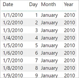
Figure 2-10 This example shows how to extract date information using date and time functions.

Relational functions

Two useful functions that you can use to navigate through relationships inside a DAX formula are RELATED and RELATEDTABLE.

You already know that a calculated column can reference column values of the table in which it is defined. Thus, a calculated column defined in Sales can reference any column of Sales. However, what if one must refer to a column in another table? In general, one cannot use columns in other tables unless a relationship is defined in the model between the two tables. If the two tables share a relationship, you can use the RELATED function to access columns in the related table.

For example, one might want to compute a calculated column in the Sales table that checks whether the product that has been sold is in the “Cell phones” category and, in that case, apply a reduction factor to the standard cost. To compute such a column, one must use a condition that checks the value of the product category, which is not in the Sales table. Nevertheless, a chain of relationships starts from Sales, reaching Product Category through Product and Product Subcategory, as shown in Figure 2-11.

Figure 2-11 Sales has a chained relationship with Product Category.

Regardless of how many steps are necessary to travel from the original table to the related table, DAX follows the complete chain of relationships, and it returns the related column value. Thus, the formula for the AdjustedCost column can look like this:

Sales[AdjustedCost] =
IF (
    RELATED ( 'Product Category'[Category] ) = "Cell Phone",
    Sales[Unit Cost] * 0.95,
    Sales[Unit Cost]
)

In a one-to-many relationship, RELATED can access the one-side from the many-side because in that case, only one row in the related table exists, if any. If no such row exists, RELATED returns BLANK.

If an expression is on the one-side of the relationship and needs to access the many-side, RELATED is not helpful because many rows from the other side might be available for a single row. In that case, we can use RELATEDTABLE. RELATEDTABLE returns a table containing all the rows related to the current row. For example, if we want to know how many products are in each category, we can create a column in Product Category with this formula:

'Product Category'[NumOfProducts] = COUNTROWS ( RELATEDTABLE ( Product ) )

For each product category, this calculated column shows the number of products related, as shown in Figure 2-12.

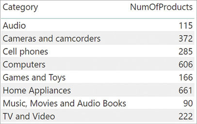
Figure 2-12 You can count the number of products by using RELATEDTABLE.

As is the case for RELATED, RELATEDTABLE can follow a chain of relationships always starting from the one-side and going toward the many-side. RELATEDTABLE is often used in conjunction with iterators. For example, if we want to compute the sum of quantity multiplied by net price for each category, we can write a new calculated column as follows:

'Product Category'[CategorySales] =
SUMX (
    RELATEDTABLE ( Sales ),
    Sales[Quantity] * Sales[Net Price]
)

The result of this calculated column is shown in Figure 2-13.

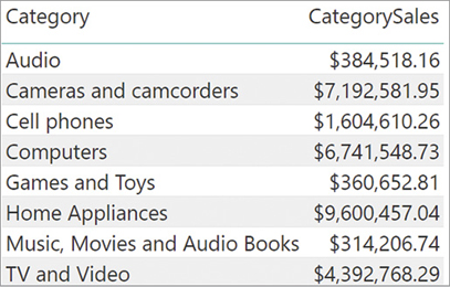
Figure 2-13 Using RELATEDTABLE and iterators, we can compute the amount of sales per category.

Because the column is calculated, this result is consolidated in the table, and it does not change according to the user selection in the report, as it would if it were written in a measure.