Unleashing the power of Excel with VBA

Understanding shortcomings of the macro recorder

Suppose you work in an accounting department. Each day you receive a text file from the company system showing all the invoices produced the prior day. This text file has commas separating the fields. The columns in the file are Invoice Date, Invoice Number, Sales Rep Number, Customer Number, Product Revenue, Service Revenue, and Product Cost (see Figure 1-8).

FIGURE 1-8 The Invoice.txt file has seven columns separated by commas.

Each morning, you manually import this file into Excel. You add a total row to the data, bold the headings, and then print the report for distribution to a few managers.

This seems like a simple process that would be ideally suited to using the macro recorder. However, due to some problems with the macro recorder, your first few attempts might not be successful. The following example explains how to overcome these problems.

CASE STUDY: PREPARING TO RECORD A MACRO

The task mentioned in the preceding section is perfect for a macro. However, before you record a macro, think about the steps you will use. In this case, the steps are as follows:

1. Click the File menu and select Open.

2. Navigate to the folder where Invoice.txt is stored.

3. Select All Files (*.*) from the Files of Type drop-down menu.

4. Select Invoice.txt.

5. Click Open.

6. In the Text Import Wizard—Step 1 Of 3 dialog box, select Delimited from the Original Data Type section.

7. Click Next.

8. In the Text Import Wizard—Step 2 Of 3 dialog box, clear the Tab key and select Comma in the Delimiters section.

9. Click Next.

10. In the Text Import Wizard—Step 3 Of 3 dialog box, select General in the Column Data Format section and change it to Date: MDY.

11. Click Finish to import the file.

12. Press the Ctrl key and the down arrow key to move to the last row of data.

13. Press the down arrow one more time to move to the total row.

14. Type the word Total.

15. Press the right arrow key four times to move to column E of the total row.

16. Click the AutoSum button and press Ctrl+Enter to add a total to the Product Revenue column while remaining in that cell.

17. Click the AutoFill handle and drag it from column E to column G to copy the total formula to columns F and G.

18. Highlight row 1 and click the Bold icon on the Home tab to set the headings in bold.

19. Highlight the total row and click the Bold icon on the Home tab to set the totals in bold.

20. Press Ctrl+* to select the current region.

21. From the Home tab, select Format, AutoFit Column Width.

After you have rehearsed these steps in your head, you are ready to record your first macro. Open a blank workbook and save it with a name such as MacroToImportInvoices.xlsm. Click the Record Macro button on the Developer tab.

In the Record Macro dialog box, the default macro name is Macro1. Change this to something descriptive like ImportInvoice. Make sure that the macros will be stored in This Workbook. You might want an easy way to run this macro later, so type the letter i in the Shortcut Key field. In the Description field, add a little descriptive text to tell what the macro is doing (see Figure 1-9). Click OK when you are ready.

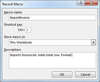
FIGURE 1-9 Before recording the macro, you need to complete the Record Macro dialog box.

Recording the macro

The macro recorder is now recording your every move. For this reason, perform your steps in exact order without extraneous actions. If you accidentally move to column F, type a value, clear the value, and then move back to E to enter the first total, the recorded macro will blindly make that same mistake day after day after day. Recorded macros move fast, but there is nothing like watching the macro recorder play out your mistakes repeatedly.

Carefully execute all the actions necessary to produce the report. After you have performed the final step, click the Stop Recording button in the Developer tab of the ribbon.

Examining code in the Programming window

Let’s look at the code you just recorded in the “Preparing to record a macro” section. Don’t worry if it doesn’t make sense yet.

To open the VB Editor, press Alt+F11. In your VBA project (MacroToImportInvoices.xlsm), find the component Module1, right-click the module, and select View Code. Notice that some lines start with an apostrophe; these are comments and are ignored by the program. The macro recorder starts your macros with a few comments, using the description you entered in the Record Macro dialog box. The comment for the keyboard shortcut is there to remind you of the shortcut.

Application.MacroOptions Macro:="ImportInvoice", _
 Description:="", ShortcutKey:="j"

Recorded macro code is usually pretty tidy (see Figure 1-10). Each line of code that is not a comment is indented 4 characters. If a line is longer than 100 characters, the recorder breaks it into multiple lines and indents the continued lines an additional 4 characters. To continue a line of code, type a space and an underscore at the end of the first line and then continue the code on the next line. Don’t forget the space before the underscore. Using an underscore without the preceding space causes an error.

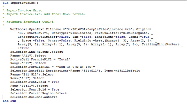
FIGURE 1-10 The recorded macro is neat looking and nicely indented.

Consider that the following seven lines of recorded code are actually only one line of code that has been broken into seven lines for readability:

Workbooks.OpenText Filename:="C:\somepath\invoice.txt", _
 Origin:=437, StartRow:=1, DataType:=xlDelimited, _
 TextQualifier:=xlDoubleQuote, ConsecutiveDelimiter:=False, _
 Tab:=True, Semicolon:=False, Comma:=True, Space:=False, _
 Other:=False, FieldInfo:=Array(Array(1, 3), Array(2, 1), _
 Array(3, 1), Array(4, 1), Array(5, 1), Array(6, 1), _
 Array(7, 1)), TrailingMinusNumbers:=True

Counting this as one line, the macro recorder was able to record the 21-step process in 14 lines of code, which is pretty impressive.

Test each macro

It is always a good idea to test macros. To test your new macro, return to the regular Excel interface by pressing Alt+F11. Close Invoice.txt without saving any changes. MacroToImportInvoices.xls is still open.

Press Ctrl+I to run the recorded macro. It should work beautifully if you completed the steps correctly. The data is imported, totals are added, bold formatting is applied, and the columns are made wider. This seems like a perfect solution (see Figure 1-11).

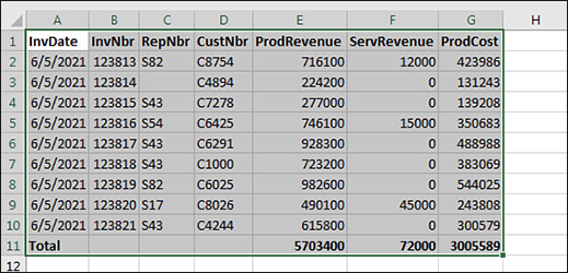
FIGURE 1-11 The macro formats the data in the sheet.

Running the macro on another day produces undesired results

After testing the macro, be sure to save your macro file to use on another day. But suppose that the next day, after receiving a new Invoice.txt file from the system, you open the macro and press Ctrl+I to run it, and disaster strikes. The data for June 5 happened to have 9 invoices, but the data for June 6 now has 17 invoices. The recorded macro blindly added the totals in Row 11 because this was where you put the totals when the macro was recorded (see Figure 1-12).

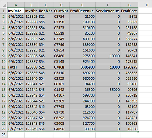
FIGURE 1-12 The intent of the recorded macro was to add a total at the end of the data, but the recorder made a macro that always adds totals at row 11.

For those of you working along using the sample files in this book, follow these steps to try importing data for another day:

1. Close Invoice.txt in Excel.

2. In Windows Explorer, rename Invoice.txt to be Invoice1.txt.

3. In Windows Explorer, rename Invoice2.txt to be Invoice.txt.

4. Return to Excel and the MacroToImportInvoices.xlsm workbook.

5. Press Ctrl+I to run the macro with the larger data set.

This problem arises because the macro recorder is recording all your actions in Absolute mode by default. As an alternative to using the default state of the macro recorder, the next section discusses relative recording and how it might get you closer to the desired solution.

Possible solution: Use relative references when recording

By default, the macro recorder records all actions as absolute actions. If you navigate to row 11 when you record the macro, the macro will always go to row 11 when the macro is run. This is rarely appropriate when dealing with variable numbers of rows of data. The better option is to use relative references when recording.

Macros recorded with absolute references note the actual address of the cell pointer, such as A11. Macros recorded with relative references note that the cell pointer should move a certain number of rows and columns from its current position. For example, if the cell pointer starts in cell A1, the code ActiveCell.Offset(16, 1).Select would move the cell pointer to B17, which is the cell 16 rows down and 1 column to the right.

Although relative recording is appropriate in most situations, there are times when you need to do something absolute while recording a macro. Here’s a great example: After adding the totals to a data set, you need to return to row 1. If you simply click row 1 while in Relative mode, Excel records that you want to select the row 10 rows above the current row. This works with the first invoice file but not with longer or shorter invoice files. Here are two workarounds:

• Toggle relative recording off, click row 1, and then toggle relative recording back on.

• Keep relative recording turned on. Display the Go To dialog box by pressing F5. Type A1 and click OK. The Go To dialog box gets recorded as always, going to the absolute address you typed, even if relative recording is turned on. A variation of this method is used in the following example.

The next example shows the same task as before but uses relative references this time. The solution will be much closer to working correctly.

CASE STUDY: RECORDING A MACRO WITH RELATIVE REFERENCES

Let’s try to record the macro again, this time using relative references.

Note: If you are following along with the sample files, complete these steps:

1. Close Invoice.txt in Excel.

2. Rename Invoice.txt as Invoice2.txt.

3. Rename Invoice1.txt as Invoice.txt.

4. Return to the MacroToImportInvoices.xlsm workbook.

In the Developer tab, choose Use Relative References to toggle on relative recording. This setting persists until you turn it off or until you close Excel.

In the workbook MacroToImportInvoices.xlsm, record a new macro by selecting Record Macro from the Developer tab. Give the new macro the name ImportInvoicesRelative and assign a different shortcut key, such as Ctrl+J.

Repeat steps 1 through 11 from the “Preparing to record a macro” section to import the file and then follow these steps:

1. Press Ctrl+down arrow to move to the last row of data.

2. Press the down arrow key one more time to move to the total row.

3. Type the word Total.

4. Press the right arrow key four times to move to column E of the total row.

5. Hold the Shift key while pressing the right arrow key twice to select E11:G11.

6. Click the AutoSum button.

7. Press Shift+spacebar to select the entire row. Type Ctrl+B to apply bold formatting to it.

8. Press F5 to display the Go To dialog box.

9. In the Go To dialog box, type A1:G1 and click OK. Even though relative recording is turned on, any navigation through the Go To dialog box is recorded as an absolute reference.

10. Click the Bold icon to set the headings in bold.

11. Press Ctrl+* to select all data in the current region.

12. From the Home tab, select Format, AutoFit Column Width.

13. Stop recording.

Press Alt+F11 to go to the VB Editor to review your code. The new macro appears in Module1, below the previous macro.

If you close Excel between recording the first and second macros, Excel inserts a new module called Module2 for the newly recorded macro:

Sub ImportInvoicesRelative()
' ImportInvoicesRelative Macro
' Import. Total Row. Format.
' Keyboard Shortcut: Ctrl+J
Workbooks.OpenText Filename:="C:\data\invoice.txt", _
 Origin:= 437, StartRow:=1, DataType:=xlDelimited, _
 TextQualifier:=xlDoubleQuote, ConsecutiveDelimiter:=False, _
 Tab:=False, Semicolon:=False, Comma:=True, Space:=False, _
 Other:=False, FieldInfo:=Array(Array(1, 3), Array(2, 1), _
 Array(3, 1), Array(4, 1), Array(5, 1), Array(6, 1), _
 Array(7, 1)), TrailingMinusNumbers:=True
Selection.End(xlDown).Select
ActiveCell.Offset(1, 0).Range("A1").Select
ActiveCell.FormulaR1C1 = "Total"
ActiveCell.Offset(0, 4).Range("A1:C1").Select
Selection.FormulaR1C1 = "=SUM(R[-9]C:R[-1]C)"
ActiveCell.Rows("1:1").EntireRow.Select
ActiveCell.Activate
Selection.Font.Bold = True
Application.Goto Reference:="R1C1:R1C7"
Selection.Font.Bold = True
Selection.CurrentRegion.Select
Selection.Columns.AutoFitSelection.Font.Bold = True
End Sub

To test the macro, close Invoice.txt without saving and then run the macro with Ctrl+J. Everything should look good, and you should get the same results as with the macro you created with the macro recorder.

The next test is to see whether the program works on the next day when you might have more rows. If you are working along with the sample files, close Invoice.txt in Excel. Rename Invoice.txt to Invoice1.txt. Rename Invoice2.txt to Invoice.txt.

Open MacroToImportInvoices.xls and run the new macro with Ctrl+J. This time, everything should look good, with the totals in the correct places. Look at Figure 1-13. Do you see anything out of the ordinary?

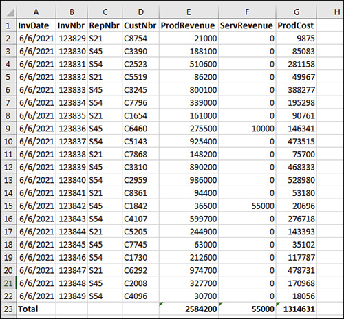
FIGURE 1-13 After running the Relative macro, the totals appear in the correct row.

If you aren’t careful, you might print these reports for your manager. If you did, you would be in trouble. When you look in cell E19, you can see that Excel has inserted a green triangle to tell you to look at the cell.

When you move the cell pointer to E19, an alert indicator pops up near the cell. This indicator tells you that the formula fails to include adjacent cells. If you look in the formula bar, you see that the macro totaled only from row 10 to row 18. Neither the relative recording nor the nonrelative recording is smart enough to replicate the logic of the AutoSum button.

Imagine that you had fewer invoice records on this particular day. Excel would have rewarded you with the illogical formula =SUM(E6:E1048574), as shown in Figure 1-14. Since this formula would be in E7, circular reference warnings appear in the status bar.

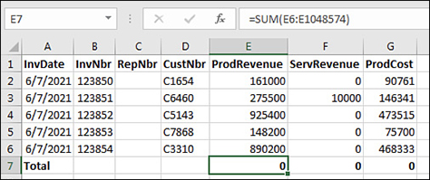
FIGURE 1-14 An incorrect formula appears when you run the relative macro with fewer invoice records.

NOTE

To try this yourself, close Invoice.txt in Excel. Rename Invoice.txt to Invoice2.txt. Rename Invoice4.txt to Invoice.txt.

If you have tried using the macro recorder, most likely you have run into problems similar to the ones produced in the previous two case studies. Although this is frustrating, you should be happy to know that the macro recorder actually gets you 95% of the way to a useful macro.

Your job is to recognize where the macro recorder is likely to fail and then be able to dive into the VBA code to fix the one or two lines that require adjusting to have a perfect macro. With some added human intelligence, you can produce awesome macros to speed up your daily work.

If you are like me, you are cursing Microsoft about now. We have wasted a good deal of time over a couple of days, and neither macro works. What makes it worse is that this sort of procedure would have been handled perfectly by the old Lotus 1-2-3 macro recorder introduced in 1983. Mitch Kapor solved this problem 33 years ago, and Microsoft still can’t get it right.

Did you know that up through Excel 97, Microsoft Excel secretly ran Lotus command-line macros? I found this out right after Microsoft quit supporting Excel 97. At that time, a number of companies upgraded to Excel XP, which no longer supported the Lotus 1-2-3 macros. Many of these companies hired my company to convert the old Lotus 1-2-3 macros to Excel VBA. It is interesting that in Excel 5, Excel 95, and Excel 97, Microsoft offered an interpreter that could handle the Lotus macros that solved this problem correctly, yet its own macro recorder couldn’t (and still can’t!) solve the problem.

Never use AutoSum or Quick Analysis while recording a macro

There actually is a macro recorder solution to the current problem with recording an AutoSum. It is important to recognize that the macro recorder will never correctly record the intent of the AutoSum button.

If you are in cell E99 and click the AutoSum button, Excel starts scanning from cell E98 upward until it locates a text cell, a blank cell, or a formula. It then proposes a formula that sums everything between the current cell and the found cell.

However, the macro recorder records the particular result of that search on the day that the macro was recorded. Rather than record something along the lines of “do the normal AutoSum logic,” the macro recorder inserts a single line of code to add up the previous 98 cells.

Excel 2013 added the Quick Analysis feature. Select E2:G99; click the Quick Analysis icon that appears below and to the right of a rectangular selection; choose Totals, Sum at Bottom; and you get the correct totals in row 100. The macro recorder hard-codes the formulas to always appear in row 100 and to always total row 2 through row 99.

The somewhat bizarre workaround is to type a SUM function that uses a mix of relative and absolute row references. If you type =SUM(E$2:E10) while the macro recorder is running, Excel correctly adds code that always sums from a fixed row two down to the relative reference that is just above the current cell.

Here is the resulting code, with a few comments:

Sub FormatInvoice3()
 ' FormatInvoice3 Macro
' Import. Total. Format.
' Keyboard Shortcut: Ctrl+K
Workbooks.OpenText Filename:="C:\Data\invoice.txt", _
    Origin:=437, StartRow:=1, DataType:=xlDelimited, _
    TextQualifier:=xlDoubleQuote, ConsecutiveDelimiter:=False, _
     Tab:=False, Semicolon:=False, Comma:=True, Space:=False, _
     Other:=False, FieldInfo:=Array(Array(1, 3), Array(2, 1), _
     Array(3, 1), Array(4, 1), Array(5, 1), Array(6, 1), _
     Array(7, 1)), TrailingMinusNumbers:=True
Selection.End(xlDown).Select
ActiveCell.Offset(1, 0).Range("A1").Select
ActiveCell.FormulaR1C1 = "Total"
ActiveCell.Offset(0, 4).Range("A1").Select
Selection.FormulaR1C1 = "=SUM(R2C:R[-1]C)"
Selection.AutoFill Destination:=ActiveCell.Range("A1:C1"), _
     Type:=xlFillDefault
ActiveCell.Range("A1:C1").Select
ActiveCell.Rows("1:1").EntireRow.Select
ActiveCell.Activate
Selection.Font.Bold = True
Application.Goto Reference:="R1C1:R1C7"
Selection.Font.Bold = True
Selection.CurrentRegion.Select
Selection.Columns.AutoFit
End Sub

This third macro consistently works with a data set of any size.

Four tips for using the macro recorder

You will rarely be able to record 100% of your macros and have them work. However, you will get much closer by using the following four tips.

Tip 1: Turn on the Use Relative References setting

Microsoft should have made this setting the default. Turn the setting on and leave it on while recording your macros.

Tip 2: Use special navigation keys to move to the bottom of a data set

If you are at the top of a data set and need to move to the last cell that contains data, you can press Ctrl+down arrow or press the End key and then the down arrow key.

Similarly, to move to the last column in the current row of the data set, press Ctrl+right arrow or press End and then press the right arrow key.

By using these navigation keys, you can jump to the end of the data set, no matter how many rows or columns you have today.

Use Ctrl+* to select the current region around the active cell. Provided that you have no blank rows or blank columns in your data, this key combination selects the entire data set.

Tip 3: Never touch the AutoSum icon while recording a macro

The macro recorder does not record the “essence” of the AutoSum button. Instead, it hard-codes the formula that resulted from pressing the AutoSum button. This formula does not work any time you have more or fewer records in the data set.

Instead, type a formula with a single dollar sign, such as =SUM(E$2:E10). When this is done, the macro recorder records the first E$2 as a fixed reference and starts the SUM range directly below the row 1 headings. Provided that the active cell is E11, the macro recorder recognizes E10 as a relative reference pointing directly above the current cell.

Tip 4: Try recording different methods if one method does not work

There are often many ways to perform tasks in Excel. If you encounter buggy code from one method, try another method. With 16 different project managers on the Excel team, it is likely that each method was programmed by a different group. In one of the case studies in this chapter, one task involved applying AutoFit Column Width to all cells. Some people might press Ctrl+A to select all cells. Others might press Ctrl+*. Since Excel 2007, the code generated by Ctrl+A when pressed in Relative mode does not work. The Ctrl+* code is very old and continues to work in all cases.