Grouping, sorting, and filtering pivot data

Sorting in a pivot table

Items in the row area and column area of a pivot table are sorted in ascending order by any custom list first. This allows weekday and month names to sort into Monday, Tuesday, Wednesday, … instead of the alphabetical order Friday, Monday, Saturday, …, Wednesday.

If the items do not appear in a custom list, they will be sorted in ascending order. This is fine, but in many situations, you want the customer with the largest revenue to appear at the top of the list. When you sort in descending order using a pivot table, you are setting up a rule that controls how that field is sorted, even after new fields are added to the pivot table.

Sorting customers into high-to-low sequence based on revenue

Three pivot tables appear in Figure 4-6. The first pivot table shows the default sort for a pivot table: Customers are arranged alphabetically, starting with Adaept, Calleia, and so on.

Figure 4-6 When you override the default sort, Excel remembers the sort as additional fields are added.

In the second pivot table, the report is sorted in descending sequence by Total Revenue. This pivot table was sorted by selecting cell E3 and choosing the ZA icon in the Data tab of the ribbon. Although that sounds like a regular sort, it is better. When you sort inside a pivot table, Excel sets up a rule that will be used after you make additional changes to the pivot table.

The pivot table in columns G:H shows what happens after you add Sector as a new outer row field. Within each sector, the pivot table continues to sort the data in descending order by revenue. Within Consulting, Surten Excel appears first, with $750K, followed by NetCom, with $614K.

You could remove Customer from the pivot table, do more adjustments, and then add Customer back to the column area, and Excel would remember that the customers should be presented from high to low.

If you could see the entire pivot table in G3:H35 in Figure 4-6, you would notice that the sectors are sorted alphabetically. It might make more sense, though, to put the largest sectors at the top. The following tricks can be used for sorting an outer row field by revenue:

• You can select cell G4 and then use Collapse Field on the Analyze tab to hide the customer detail. When you have only the sectors showing, select H4 and click ZA to sort descending. Excel understands that you want to set up a sort rule for the Sector field.

• You can temporarily remove Customer from the pivot table, sort descending by revenue, and then add Customer back.

• You can use More Sort Options, as described in the following paragraphs.

To sort the Sector field, you should open the drop-down menu for the Sector field. Hover over Sector in the top of the PivotTable Fields list, and click the drop-down arrow that appears (see Figure 4-7). Or, if your pivot table is shown in Tabular layout or Outline layout, you can simply open the drop-down arrow in cell G3.

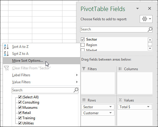
FIGURE 4-7 For explicit control over sort order, open this drop-down menu.

Inside the drop-down menu, choose More Sort Options to open the Sort (Sector) dialog box. In this dialog box, you can choose to sort the Sector field in Descending order by Total $ (see Figure 4-8).

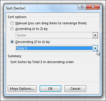
FIGURE 4-8 Choose to sort Sector based on the Total $ field.

The Sort (Sector) dialog box shown in Figure 4-8 includes a More Options button in the lower left. If you click this button, you arrive at the More Sort Options dialog box, in which you can specify a custom list to be used for the first key sort order. You can also specify that the sorting should be based on a column other than Grand Total.

In Figure 4-10, the pivot table includes Product in the column area. If you wanted to sort the customers based on total gadget revenue instead of total revenue, for example, you could do so with the More Sort Options dialog box. Here are the steps:

1. Open the Customer heading drop-down menu in B4.

2. Choose More Sort Options.

3. In the Sort (Customer) dialog box, choose More Options.

4. In the More Sort Options (Customer) dialog box, choose the Sort By Values In Selected Column option (see Figure 4-9).

5. Click in the reference box and then click cell D5. Note that you cannot click the Gadget heading in D4; you have to choose one of the Gadget value cells.

6. Click OK twice to return to the pivot table.

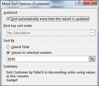
FIGURE 4-9 Using More Sort Options, you can sort by a specific pivot field item.

If your pivot table has only one field in the Rows area, you can set up the “Sort by Doodads” rule by doing a simple sort using the Data tab. Select any cell in B5:B30 and choose Data, ZA. The pivot table will be sorted with the largest Doodads customers at the top (see Figure 4-10). Note that you cannot sort from the Doodads heading in B4. Sorting from there will sort the product columns by revenue.

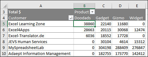
FIGURE 4-10 Sort from cell E5 to sort by Doodads.

Using a manual sort sequence

The Sort dialog box offers something called a manual sort. Rather than using the dialog box, you can invoke a manual sort in a surprising way.

Note that the products in Figure 4-10 are in the following order: Doodads, Gadget, Gizmo, and Widget. It appears that the Doodads product line is a minor product line and probably would not fall first in the product list.

Place the cell pointer in cell E4 and type the word Doodads. When you press Enter, Excel figures out that you want to move the Doodads column to be last. All the values for this product line move from column B to column E. The values for the remaining products shift to the left.

One unintended consequence is that the customers re-sort based on the product that moved to column B: Gadget. This is because the “Sort by Doodads” rule was actually a “Sort by whatever is in column B” rule.

In Figure 4-11, note the numbers in row 17 and compare them to the numbers in row 5 in Figure 4-10. The values followed the change in headings.

FIGURE 4-11 Simply type a heading in E4 to rearrange the columns.

This behavior is completely unintuitive. You should never try this behavior with a regular (non–pivot table) data set in Excel. You would never expect Excel to change the data sequence just by moving the labels. Figure 4-11 shows the pivot table after a new column heading has been typed in cell E4.

If you prefer to use the mouse, you can drag and drop the column heading to a new location. Select a column heading. Hover over the edge of the active cell border until the mouse changes to a four-headed arrow. Drag the cell to a new location, as shown in Figure 4-12. When you release the mouse, all the value settings move to the new column.

FIGURE 4-12 Use drag and drop to move a column to a new position.

Using a custom list for sorting

Another way to permanently change the order of items along a dimension is to set up a custom list. All future pivot tables created on your computer will automatically respect the order of the items in a custom list.

The pivot table at the top of Figure 4-13 includes weekday names. The weekday names were added to the original data set by using =TEXT(F2,"DDD") and copying down. Excel automatically puts Sunday first and Saturday last, even though this is not the alphabetical sequence of these words. This happens because Excel ships with four custom lists to control the days of the week, months of the year, and the three-letter abbreviations for both.

FIGURE 4-13 The weekday names in B4:H4 follow the order specified in the Custom Lists dialog box.

You can define your own custom list to control the sort order of pivot tables. Follow these steps to set up a custom list:

1. In an out-of-the-way section of the worksheet, type the products in their proper sequence. Type one product per cell, going down a column.

2. Select the cells containing the list of regions in the proper sequence.

3. Click the File tab and select Options.

4. Select the Advanced category in the left navigation bar. Scroll down to the General group and click the Edit Custom Lists button. In the Custom Lists dialog box, your selection address is entered in the Import text box, as shown in Figure 4-13.

5. Click Import to bring the products in as a new list.

6. Click OK to close the Custom Lists dialog box, and then click OK to close the Excel Options dialog box.

The custom list is now stored on your computer and is available for all future Excel sessions. All future pivot tables will automatically show the product field in the order specified in the custom list. Figure 4-14 shows a new pivot table created after the custom list was set up.

FIGURE 4-14 After you define a custom list, all future pivot tables will follow the order in the list.

To sort an existing pivot table by the newly defined custom list, follow these steps:

1. Open the Product header drop-down menu and choose More Sort Options.

2. In the Sort (Product) dialog box, choose More Options.

3. In the More Sort Options (Product) dialog box, clear the AutoSort check box.

4. As shown in Figure 4-15, in the More Sort Options (Product) dialog box, open the First Key Sort Order drop-down menu and select the custom list with your product names.

5. Click OK twice.

FIGURE 4-15 Choose to sort by the custom list.