Query and transform data
- By Daniil Maslyuk and Justin Frebault
- 12/24/2023
- Skill 2.1: Query data by using Azure Synapse Analytics
- Skill 2.2: Ingest and transform data by using Power BI
In this sample chapter from Exam Ref DP-500 Designing and Implementing Enterprise-Scale Analytics Solutions Using Microsoft Azure and Microsoft Power BI, you will learn how data is queried and transformed with Azure Synapse and Power BI. This chapter covers Skills 2.1 and 2.2 from the DP-500 exam.
Data duplication is natural in an organization. Data needs to be queried and transformed in a format that is most suitable for the use case. This is true even at the lowest level, in a database, where data is duplicated in the form of indexes to optimize reads.
Similarly, in an organization data will be queried and transformed from the operational to the analytical system(s), and queried and transformed again through the various layers of the analytical stack. In this chapter we will review how this is done with Azure Synapse and Power BI.
Skills covered in this chapter:
2.1: Query data by using Azure Synapse Analytics
2.2: Ingest and transform data by using Power BI
Skill 2.1: Query data by using Azure Synapse Analytics
There is no doubt that the amount of data generated and used by businesses is growing. And so are the requirements for near-real-time analytics; we want more insight and sooner. On top of that, the complexity of the analysis is increasing. With predictive and prescriptive solutions, we go beyond descriptive and diagnostic analytics.
To meet all these increasingly demanding requirements, data tools are multiplying. But there is value in a single platform: ease of training, reduced cognitive load, easier cross-team collaboration, fewer silos in the organization. . . . Azure Synapse Analytics is all about bringing together data engineers, data scientists, and data analysts in order to achieve more with your data.
Identify an appropriate Azure Synapse pool when analyzing data
Azure Synapse Analytics is an extremely rich platform (see Figure 2-1). As the requirements around data become more and more complex, so does the need for features. Azure Synapse Analytics can be seen as a one-stop shop for data in your organization, bringing together data engineers, data scientists, and data analysts.
)
FIGURE 2.1 Overall architecture diagram of Azure Synapse Analytics
Overall architecture of Azure Synapse Analytics
In Chapter 1, we reviewed the tight integration with Microsoft Purview, and with Power BI. Azure Synapse Analytics comes with a default data store: the Azure Data Lake Storage Gen2, although it is possible to link more data stores to your Azure Synapse Analytics. The default data store supports Delta Lake, an open source storage layer that comes on top of the Data Lake Storage and brings ACID transactions to Apache Spark.
Azure Synapse Analytics offers two query engines: Apache Spark and SQL. We will review both technologies and their various flavors in this chapter. These query engines allow for batch processing, parallel processing, stream processing, and machine learning workload. The beauty of Azure Synapse Analytics is also the variety of languages you can work with. SQL is the first to come to mind, but there is also Scala, Python, R, and last but not least, C#. Finally, Synapse Pipelines enables data transformations, even in a parallel computing fashion, with a low code tool.
Concepts about Spark Pool
Apache Spark is a framework for in-memory parallel processing. It was first released in 2014, with the goal to provide a unified platform for data engineering and data science, as well as batch and streaming—a mission that resonates with Azure Synapse Analytics. Apache Spark is originally written in Scala, but also available in Python, SQL, and R. In Azure Synapse Analytics, Apache Spark is also available in C#.
Apache Spark runs on a cluster, as you can see in Figure 2-2.
)
FIGURE 2.2 High-level overview of a Spark cluster
A Spark application is coordinated by the driver program. On a cluster, the driver program connects to the cluster manager to coordinate the work. In Azure Synapse Analytics, the cluster manager is YARN. The cluster manager is responsible for allocating resources (memory, cores, etc.) in the cluster. Once the driver is connected to the cluster manager, it acquires resources to create executors. Executors will be the ones doing the work: running in-memory computations and storing data.
An Azure Spark pool is not just a Spark instance on a cluster. Azure Synapse provides peripheral features:
Auto-Scale capabilities—The Auto-Scale feature automatically scales up and down the number of nodes in a cluster. You can set a minimum and maximum number of nodes when creating a new Spark pool. Every 30 seconds, Auto-Scale monitors the number of CPUs and the amount of memory needed to complete all pending jobs, as well as the current total CPUs and memory, and scales up or down based on these metrics.
Apache Livy—Apache Livy is a REST API for Apache Spark. Conveniently, it is included in Azure Spark pools. Apache Livy can be used to submit programmatically Spark jobs to the cluster.
Preloaded Anaconda libraries—Apache Spark is great for parallel computing, but sometimes we don’t need all that computing power, but instead want some more specialized functionalities for machine learning or visualization. Particularly during exploratory analysis, having Anaconda libraries preloaded in Azure Spark pools comes in handy.
An Azure Spark pool is a great tool when dealing with a large amount of data and when performance matters. Should it be data preparation, machine learning, or streaming data, a Spark pool is the right tool if you want to work in Python, SQL, Scala, or C#.
Example of how to use it
To review how to use an Azure Spark pool, we will start by creating an Azure Synapse Analytics resource.
In your Azure portal, select Create a resource.
Search for and select Azure Synapse Analytics.
Select Create.
Once the resource is created, navigate to the resource and select Open Synapse Studio, as shown in Figure 2-3.
)
FIGURE 2.3 Synapse Resource view in the Azure portal
Now that we have our resource, let’s create the Spark pool.
Go to Manage, as shown in Figure 2-4.

FIGURE 2-4 The Manage menu in Azure Synapse Analytics Studio
Navigate to Apache Spark pools > + New.
Enter a name in Apache Spark pool name, like dp500.
Set Isolated compute to Disabled.
Set Node size family as Memory Optimized.
Set Node size to Small.
Set Autoscale to Enabled.
Set Number of nodes to 3 and 5.
Review that you have the same configuration as Figure 2-5.
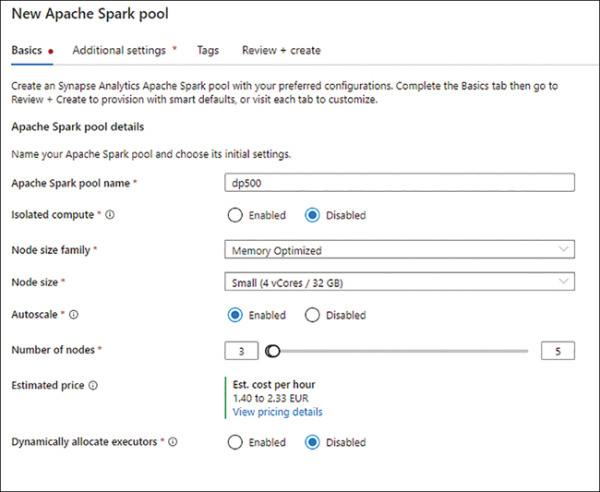
FIGURE 2.5 Configuration parameters for the Apache Spark pool
Select Review + create.
Select Create.
)
)
Now that we have our compute, we can use it to query and analyze some data. To do that, we first need to get some data.
Navigate to https://www.nyc.gov/site/tlc/about/tlc-trip-record-data.page and download the January 2022 Green Taxi Trip Records.
In the Synapse Studio, navigate to the Data menu, as shown in Figure 2-6.
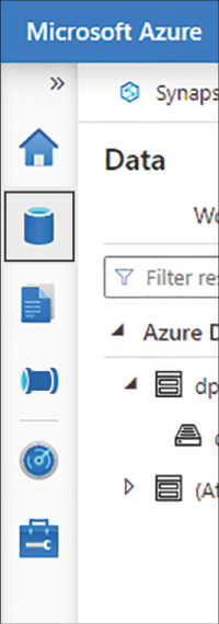
FIGURE 2-6 Data menu in Synapse Studio
Select the Linked tab and then select Azure Data Lake Storage Gen2.
Expand your primary container and select your primary file store.
Upload your Parquet file.
Right-click on the uploaded file and from the context menu select New notebook > Load to Dataframe.
In the new notebook, attach the Spark pool you created previously.
Run the first cell.
)
After a few minutes, the time for the Spark pool to spin up, you should see a table with the first 10 rows of the dataset, as shown in Figure 2-7. The data is now loaded in memory in a Spark DataFrame, so the analysis can proceed.
)
FIGURE 2.7 Results from reading the Parquet file with the Spark pool
Architecture of Synapse SQL
Before diving into the two flavors of Azure Synapse SQL, let’s review the overall architecture of this part of Azure Synapse Analytics. Figure 2-8 represents the internal architecture of Azure Synapse SQL.
)
FIGURE 2.8 The internal architecture of Azure Synapse SQL
The control node is going to be the entry point of Azure Synapse SQL and the orchestrator of the distributed query to the compute node, similar to the driver node in a Spark pool. And as their name indicates, the compute nodes will do the computation.
It is important to note the decoupling of compute and storage, which will also be reflected in the pricing. You can scale your compute without affecting your storage, and vice versa.
The difference between serverless and dedicated is primarily in the number of nodes available. With serverless, the number of nodes is not predetermined and will scale automatically based on the computation needs. With dedicated, the number of nodes is preallocated.
A dedicated SQL pool also, beyond querying the data, allows ingestion of data, whereas serverless only allows querying the data. The ingestion of data will allow you to create tables in your SQL pool. Those tables will be distributed. There are three possible distributions: hash, round-robin, and replicate.
The hash distribution is typically used for large tables, such as fact tables. The round-robin is used for staging tables. And the replicate is used for small tables, such as dimensions.
 EXAM TIP
You will often find questions about the optimal distribution for a use case. So it’s important that you thoroughly understand each of the three distributions and when they would be appropriate to use.
SQL serverless pool
Because a SQL serverless pool is serverless, that doesn’t mean there is no server behind the scene, but it does mean that for you there is no infrastructure to set up or maintain. A SQL serverless pool will be automatically provisioned and ready to go when you create a Synapse Analytics workspace, and it will scale as needed. You will be charged by how much data you process.
Because of that, a SQL serverless pool is particularly suited for unpredictable workloads, such as exploratory analysis. Another perfect use case for SQL serverless pools is to create a logical data warehouse, to be queried by Power BI. Indeed, instead of provisioning a cluster so that Power BI can query your data lake, a SQL serverless pool is available whenever you need it.
Example of how to use it
To see how to use SQL serverless pools, let’s open our Synapse Studio:
Go to the Develop menu, as shown in Figure 2-9.

FIGURE 2-9 Develop menu in Synapse Studio
Select + > SQL script, as shown in Figure 2-10.
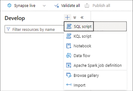
FIGURE 2-10 The Develop menu with its various capabilities
In the menu above the first line of the script, verify that you are connected to the Built-in compute. Built-in is the name of the SQL serverless pool automatically created for you when you create an Azure Synapse Analytics resource.
Using the OPENROWSET function, query the previously loaded taxi dataset, and display the top 10 rows:
SELECT TOP 10 *
FROM OPENROWSET(
        BULK 'https://yoursynapseresource.dfs.core.windows.net/yourfilestore/
synapse/workspaces/green_tripdata_2022-01.parquet',
FORMAT = 'PARQUET' ) AS [result]
Select Run.
)
)
After a few seconds—the start-up time is much less than for the Apache Spark pool—you should see a table with the first 10 rows of the dataset, as shown in Figure 2-11.
)
FIGURE 2.11 Results from querying the dataset with a SQL serverless pool
EXAM TIP
It is important to understand how the function OPENROWSET works and how to use it. If you need more review, please consult the documentation here: https://learn.microsoft.com/en-us/sql/t-sql/functions/openrowset-transact-sql?view=sql-server-ver16.
Concepts about SQL dedicated pools
Synapse SQL dedicated pools differ from serverless in two major ways: first, because of its dedicated nature it needs to be provisioned, and second, data can be ingested in a SQL dedicated pool.
When provisioning the pool, you will have to define its size in DWUs (data warehousing units). A DWU is an abstraction representing a unit that combines CPU, memory, and I/O.
To ingest data into the dedicated pool, you can use T-SQL to query data from external sources. This is possible thanks to PolyBase, a virtualization feature that allows you to query data from various sources without the need to install a client connection software.
Table partitioning is an important topic to review for SQL dedicated pools.
Round-Robin Distribution
Round-robin will favor data writes, not reads, so it is suitable for rapidly loading data and therefore suitable for staging tables. It randomly distributes table rows evenly across all nodes. Querying data distributed in a round-robin fashion, particularly with joins, will yield poor performance. To accomplish that, it’s better to use hash distribution.
Hash Distribution
Hash distribution won’t distribute rows randomly, but rather it will use a deterministic hash function to assign each value to a node. If two values are the same, they will be assigned to the same node. This is important to remember when choosing the column used for partitioning. If a column has skew—that is, many times the same value—one node will be a hot spot (overused) and the other nodes will barely have any data on them. So it’s important to choose a column evenly distributed. The hash distribution is typical for large fact tables. For smaller tables, like dimensions, there is a third option.
Replicated Distribution
As its name indicates, replicated distribution will copy the table in each node. That could be seen as a waste of space, but in a distributed workload that’s a huge performance boost, since data doesn’t need to move around if each node already has it. This is only possible if the table is small, so typically this distribution is used for dimension tables. The general guidance is to use replicated for tables smaller than 2 GB.
Recommend appropriate file types for querying serverless SQL pools
Synapse serverless SQL pool scales automatically and doesn’t need you to provision anything. That’s why it’s great for unpredictable workloads and logical data warehousing. You pay depending on how much data you query. Moreover, it’s important to remember that Synapse is catering for your analytics needs, not your operational needs. This affects the access patterns appropriate for Synapse serverless SQL pools. For example, an online transaction processing (OLTP) workload, updating or reading all columns of a single row, is not the appropriate use case. Analytics needs mean online analytical processing (OLAP), in other words, querying a large number of rows, on a limited number of columns, often with some aggregations performed. The ideal access pattern will be important in your choice of file to query for Synapse Analytics.
Typically three different file types can be queried with SQL serverless pools: CSV, JSON, and Parquet. CSV (comma-separated values) files are common in many businesses. JSON (JavaScript Object Notation) files are common in web applications. And Parquet files are common for analytics applications.
The syntax is the same to query them, making use of the OPENROWSET function:
SELECT *FROM OPENROWSET(
    BULK 'https://mydatalake.blob.core.windows.net/data/files/*.csv',
    FORMAT = 'csv') AS rows
Why is Parquet recommended for analytics? It comes down to the access pattern. Parquet files store the data in a columnar format, whereas JSON and CSV store files in a row format. This has two implications. First, accessing the data for OLAP queries is faster with columnar format, because the data we want to query (the whole column) is physically stored next to each other. With a CSV or JSON file, the data of the same column would be physically scattered. Second, the data is generally more homogenous in a column than in a row. Indeed, usually a row contains multiple data types, so there will be a mix of data. In a column the data has the same type and can be similar or even identical sometimes. This leads to greater potential for compression. That is why Parquet files are recommended for analytics workloads.
How to query Parquet files
To review how to query a Parquet file, let’s go back to our Synapse Studio:
Navigate to Develop > + > SQL script.
Make sure it is attached to Built-in, as a reminder, this is your serverless pool.
Using OPENROWSET, select the top 10 rows of your taxi dataset in a Parquet format:
SELECT
 TOP 10 *
FROM
OPENROWSET(
BULK 'https:// your-storage.dfs.core.windows.net/ your-filestore /synapse/
workspaces/green_tripdata_2022-01.parquet',
FORMAT = 'PARQUET'
) AS [result]
Select Run.
You should get the same results as before, as shown earlier in Figure 2-11.
Query relational data sources in dedicated or serverless SQL pools, including querying partitioned data sources
SQL pools, whether dedicated or serverless, will test your knowledge of T-SQL. Here you will learn how to query data, both with dedicated and serverless, and we will also consider partitioned data.
To review how to use SQL dedicated pools, let’s go back to our Synapse Studio and:
Go to the Manage menu.
Under Analytics pools select SQL pools > + New.
Set Dedicated SQL Pool Name to a name of your choice
Change the Performance level to DW100c; the default is DW1000c.
Select Review + create > Create.
The deployment of the dedicated SQL pool will take a few minutes. Next let’s look at how to ingest the data into the dedicated pool:
Go to Develop > + > SQL script.
Set the Connect to option to your dedicated SQL pool, not to Built-in.
You can ingest from the data lake to your SQL dedicated pool with the COPY statement. You will need to replace the file address with your own address:
COPY INTO dbo.TaxiTrips
FROM 'https://your-storage.dfs.core.windows.net/your-filestore/synapse/workspaces/
green_tripdata_2022-01.parquet'
WITH
(
FILE_TYPE = 'PARQUET',
MAXERRORS = 0,
IDENTITY_INSERT = 'OFF',
AUTO_CREATE_TABLE = 'ON'
)
You can now run a SELECT on the newly created table in your dedicated pool. You will see that the table has been populated with the data from the Parquet file.
SELECT TOP 10 * FROM dbo.TaxiTrips
Select Run.
You should now see the first 10 rows of the table, as shown in Figure 2-12.
)
FIGURE 2.12 Results from querying the populated table with Synapse Dedicated Pool
Don’t forget to pause your dedicated SQL pool to limit the cost of this exercise.
Oftentimes, though, Parquet files are partitioned. To review and reproduce this use case, we’ll use the SQL serverless pool. So follow these steps:
Navigate to https://www.nyc.gov/site/tlc/about/tlc-trip-record-data.page and download the February and March 2022 Green Taxi Trip Records.
In Synapse Studio, select Data > Linked > Azure Data Lake Storage Gen2.
Open your primary data store.
With the + New folder command, create a folder structure in your data store representing YEAR/MONTH, as shown in Figure 2-13.
)
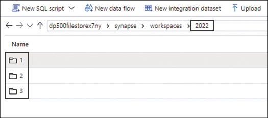
FIGURE 2-13 The file store hierarchy in Synapse Studio
Upload the datasets in their corresponding folders; you should have one Parquet file per month.
To leverage the partitioning in your query, try to count how many records are in each partition, using the OPENROWSET function, the Parquet format, and the * wildcard.
Run the query for Partitions 1 and 2:
SELECT
COUNT(*)
FROM
OPENROWSET(
BULK 'https:// your-storage.dfs.core.windows.net/ your-filestore /synapse/
workspaces/2022/*/*.parquet',
FORMAT = 'PARQUET'
) AS TaxiTrips
WHERE TaxiTrips.filepath(1) IN ('1', '2')
Run the query for Partition 1:
SELECT
COUNT(*)
FROM
OPENROWSET(
BULK 'https://your-storage.dfs.core.windows.net/your-filestore/synapse/
workspaces/2022/*/*.parquet',
FORMAT = 'PARQUET'
) AS TaxiTrips
WHERE TaxiTrips.filepath(1) IN ('1')
Check that the results are different.
You now know how to query a Parquet file containing partitions.
Use a machine learning PREDICT function in a query
Finally, Synapse SQL dedicated pools can be used to consume a machine learning model. For example, with our taxi dataset, we could have a model to predict the duration of the trip, based on the pickup location and the time of day. Having the ability to score, or consume, the model directly in Synapse Analytics is useful because we don’t need to move the data outside of our data analytics platform. To score our model, we will use the PREDICT function.
However, a Synapse SQL dedicated pool doesn’t have the ability to train a machine learning model. So to use the PREDICT function, we will need to have the model trained outside of Synapse SQL. We could, for example, train the model in a Synapse Spark pool or in another product like Azure Machine Learning.
The trained model will need to be converted to the ONNX (Open Neural Network Exchange) format. ONNX is an open source standard format, with the very purpose of enabling exchange of models between platforms.
Load a model in a Synapse SQL dedicated pool table
The model has to be stored in a dedicated SQL pool table, as a hexadecimal string in a varbinary(max) column. For instance, such a table could be created with this:
CREATE TABLE [dbo].[Models]
(
[Id] [int] IDENTITY(1,1) NOT NULL,
[Model] [varbinary](max) NULL,
[Description] [varchar](200) NULL
)
WITH
(
DISTRIBUTION = ROUND_ROBIN,
HEAP
)
GO
where Model is the varbinary(max) column storing our model, or models, as hexadecimal strings.
Once the table is created, we can load it with the COPY statement:
COPY INTO [Models] (Model)
FROM '<enter your storage location>'
WITH (
FILE_TYPE = 'CSV',
CREDENTIAL=(IDENTITY= 'Shared Access Signature', SECRET='<enter your storage key here>')
)
We now have a model ready to be used for scoring.
Scoring the model
Finally, the PREDICT function will come into play to score the model. Like any machine learning scoring, you will need the input data to have the same format as the training data.
The following query shows how to use the PREDICT function. It takes the model and the data as parameters.
DECLARE @model varbinary(max) = (SELECT Model FROM Models WHERE Id = 1);
SELECT d.*, p.Score
FROM PREDICT(MODEL = @model,
DATA = dbo.mytable AS d, RUNTIME = ONNX)
WITH (Score float) AS p;