Troubleshooting formulas

Auditing a worksheet

As you’ve seen, some formula errors result from referencing other cells that contain errors or inappropriate values. The first step in troubleshooting these formula problems is to determine which cell (or group of cells) is causing an error. This is straightforward if the formula references only a single cell, but it gets progressively more difficult as the number of references increases. (Another complicating factor is the use of range names because it won’t be obvious which range each name is referencing.)

To determine which cells are wreaking havoc on your formulas, you can use Excel’s auditing features to visualize and trace a formula’s input values and error sources.

Understanding auditing

Excel’s formula-auditing features operate by creating tracers—arrows that literally point out the cells involved in a formula. You can use tracers to find three kinds of cells:

• Precedents: These are cells that are directly or indirectly referenced in a formula. For example, suppose that cell B4 contains the formula =B2; then B2 is a direct precedent of B4. Now suppose that cell B2 contains the formula =A2/2; this makes A2 a direct precedent of B2, but it’s also an indirect precedent of cell B4.

• Dependents: These are cells that are directly or indirectly referenced by a formula in another cell. In the preceding example, cell B2 is a direct dependent of A2, and B4 is an indirect dependent of A2.

• Errors: These are cells that contain an error value and are directly or indirectly referenced in a formula (and therefore cause the same error to appear in the formula).

Figure 3-7 shows a worksheet with three examples of tracer arrows:

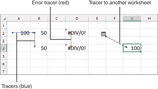
FIGURE 3-7 This worksheet demonstrates the three types of tracer arrows.

• Cell B4 contains the formula =B2, and B2 contains =A2/2. The arrows (they’re blue onscreen) point out the precedents (direct and indirect) of B4.

• Cell D4 contains the formula =D2, and D2 contains =D1/0. The latter produces the #DIV/0! error. Therefore, the same error appears in cell D4. The arrow (it’s red onscreen) is pointing out the source of the error.

• Cell G4 contains the formula =Sheet5!A1. Excel displays the dashed arrow with the worksheet icon whenever the precedent or dependent exists on a different worksheet.

Tracing cell precedents

To trace cell precedents, follow these steps:

1. Select the cell that contains the formula whose precedents you want to trace.

2. Select Formulas > Trace Precedents. Excel adds a tracer arrow to each direct precedent.

3. Keep repeating step 2 to see more levels of precedents.

Tracing cell dependents

Here are the steps to follow to trace cell dependents:

1. Select the cell whose dependents you want to trace.

2. Select Formulas > Trace Dependents. Excel adds a tracer arrow to each direct dependent.

3. Keep repeating step 2 to see more levels of dependents.

Tracing cell errors

To trace cell errors, follow these steps:

1. Select the cell that contains the error you want to trace.

2. Select Formulas > Error Checking > Trace Error. Excel adds a tracer arrow to each cell that produced the error.

Removing tracer arrows

To remove the tracer arrows, you have three choices:

• To remove all the tracer arrows, select Formulas > Remove Arrows.

• To remove precedent arrows one level at a time, select Formulas, open the Remove Arrows drop-down menu, and select Remove Precedent Arrows.

• To remove dependent arrows one level at a time, select Formulas, open the Remove Arrows drop-down menu, and select Remove Dependent Arrows.

Evaluating formulas

Earlier, you learned that you could troubleshoot a wonky formula by evaluating parts of it. You do this by selecting the part of the formula you want to evaluate and then selecting F9. This works fine, but it can be tedious in a long or complex formula, and there’s always a danger that you might accidentally confirm a partially evaluated formula and lose your work.

A better solution is to use Excel’s Evaluate Formula feature. It does the same thing as the F9 technique, but it’s easier and safer. Here’s how it works:

1. Select the cell that contains the formula you want to evaluate.

2. Select Formulas > Evaluate Formula. Excel displays the Evaluate Formula dialog box.

3. The current term in the formula is underlined in the Evaluation box. At each step, you select from one or more of the following buttons:

   • Evaluate: Display the current value of the underlined term.

   • Step In: Display the first dependent of the underlined term. If that dependent also has a dependent, select this button again to see it (see Figure 3-8).

     

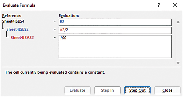
     FIGURE 3-8 With the Evaluate Formula feature, you can “step into” the formula to display its dependent cells.

   • Step Out: Hide a dependent and evaluate its precedent.

4. Repeat step 3 until you’ve completed your evaluation.

5. Select Close.

Watching cell values

In the precedent tracer example shown in Figure 3-7, the formula in cell G4 refers to a cell in another worksheet, which is represented in the trace by a worksheet icon. In other words, you can’t see the formula cell and the precedent cell simultaneously. This could also happen if the precedent existed on another workbook or even elsewhere on the same sheet if you’re working with a large model.

This is a problem because there’s no easy way to determine the current contents or value of the unseen precedent. If you’re having a problem, troubleshooting requires that you track down the far-off precedent to see if it might be the culprit. That’s bad enough with a single unseen cell, but what if your formula refers to 5 or 10 such cells? And what if those cells are scattered in different worksheets and workbooks?

This level of hassle—not uncommon in the spreadsheet world—was undoubtedly the inspiration behind an elegant solution: the Watch Window. This window enables you to keep tabs on both the value and the formula in any cell in any worksheet in any open workbook. Here’s how you set up a watch:

1. Switch to the workbook that contains the cell or cells you want to watch.

2. Select Formulas > Watch Window. Excel displays the Watch Window.

3. Select Add Watch. Excel displays the Add Watch dialog box.

4. Either select the cell you want to watch or type in a reference formula for the cell (for example, =A1). Note that you can select a range to add multiple cells to the Watch Window.

5. Select Add. Excel adds the cell or cells to the Watch Window, as shown in Figure 3-9.

   

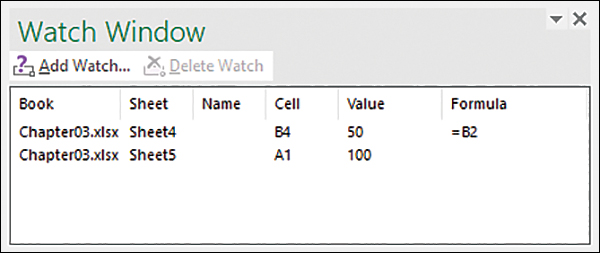
   FIGURE 3-9 Use the Watch Window to keep an eye on the values and formulas of unseen cells that reside in other worksheets or workbooks.

When you no longer need a watch, you should remove it to avoid cluttering the Watch Window. To remove a watch, select Formulas > Watch Window to open the Watch Window, select the watch, and then select Delete Watch.