Troubleshooting formulas

Fixing other formula errors

Not all formula errors generate one of Excel’s 11 error values. Instead, you might see a warning dialog box from Excel (for example, if you try to enter a function without including a required argument). Or, you might not see any indication that something is wrong. To help you in these situations, the following sections cover some of the most common formula errors.

Missing or mismatched parentheses

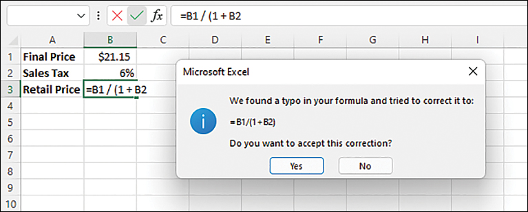
If you miss a parenthesis when typing a formula or place a parenthesis in the wrong location, Excel usually displays a dialog box like the one shown in Figure 3-1 when you attempt to confirm the formula. If the edited formula is what you want, select Yes to have Excel enter the corrected formula automatically; if the edited formula is incorrect, select No and edit the formula by hand.

FIGURE 3-1 If you miss a parenthesis, Excel attempts to fix the problem and displays this dialog box to ask if you want to accept the correction.

To help you avoid missing or mismatched parentheses, Excel provides two visual clues in the formula itself when you’re editing it:

• The first clue occurs when you type a close parenthesis character—). Excel temporarily bolds both the close parenthesis and its corresponding open parenthesis—(. If you type what you think is the last close parenthesis, but Excel doesn’t bold the first open parenthesis, your parentheses are unbalanced.

• The second clue occurs when you use the left and right arrow keys to navigate a formula. When you cross over a parenthesis, Excel bolds the other parenthesis in the pair.

Erroneous formula results

If a formula produces no warnings or error values, the result might still be in error. If the result of a formula is incorrect, here are a few techniques that can help you understand and fix the problem:

• Calculate complex formulas one term at a time. In the formula bar, select the expression you want to calculate and then press F9. Excel converts the expression into its value. Make sure that you press the Esc key when you’re done to avoid entering the formula with just the calculated values.

• Evaluate the formula. You can step through the various parts of a formula, a technique that I describe later in this chapter (see “Evaluating formulas”).

• Break up long or complex formulas. One of the most problematic aspects of formula troubleshooting is making sense out of long formulas. The previous techniques can help (by enabling you to evaluate parts of the formula), but it’s usually best to keep your formulas as short as you can at first. When you get things working properly, you can often combine formulas for a more efficient model.

• Recalculate all formulas. A formula might display the wrong result because other formulas on which it depends need to be recalculated. This is particularly true if one or more of those formulas use custom VBA functions. Select Shift+F9 to recalculate all worksheet formulas.

• Pay attention to operator precedence. As explained in Chapter 1, “Building basic formulas,” Excel’s operator precedence means that certain operations are performed before others. An erroneous formula result could, therefore, be caused by Excel’s precedence order. To control precedence, use parentheses.

• Watch out for nonblank “blank” cells. A cell might appear to be blank but actually contain data or even a formula. For example, some users “clear” a cell by selecting the spacebar, and Excel then treats the cell as nonblank. Similarly, some formulas return an empty string instead of a value. (For example, see the IF function formula earlier in this chapter for avoiding the #DIV/0! error.)

• Watch unseen values. In a large model, your formula could be using cells that you can’t see because they’re offscreen or on another sheet. Excel’s Watch Window enables you to keep an eye on the current value of one or more cells. To learn about the Watch Window, see “Watching cell values,” later in this chapter.

Fixing circular references

A circular reference occurs when a formula refers to its own cell. This can happen in one of two ways:

• Directly: The formula explicitly references its own cell. For example, a circular reference would result if the following formula were entered into cell A1:

  =A1+A2

• Indirectly: The formula references a cell or function that, in turn, references the formula’s cell. For example, suppose that cell A1 contains the following formula:

  =A5*10

• A circular reference would result if cell A5 referred to cell A1, as in this example:

  =SUM(A1:D1)

When Excel detects a circular reference, it displays the dialog box shown in Figure 3-2. Here’s the formula in cell B3:

FIGURE 3-2 If you attempt to enter a formula that contains a circular reference, Excel displays this dialog box.

=B1 / (1 + B2)

Here’s the formula in cell B1:

=B3 * (1 + B2)

These formulas refer to each other’s cells, creating a circular reference.

When you select OK, Excel displays tracer arrows that connect the cells involved in the circular reference. (Tracers are discussed in detail later in this chapter; see “Auditing a worksheet.”) Knowing which cells are involved enables you to correct the formula in one of them to solve the problem.