An Architectural Perspective of ML.NET
- By Dino Esposito and Francesco Esposito
- 3/28/2022
- Life Beyond Python
- Introducing ML.NET
- Consuming a Trained Model
- Summary
Introducing ML.NET
First released in the spring of 2019, ML.NET is a free cross-platform and open-source .NET framework designed to build and train machine learning models and host them within .NET applications. See https://dotnet.microsoft.com/apps/machinelearning-ai/ml-dotnet.
ML.NET aims to provide the same set of capabilities that data scientists and developers can find in the Python ecosystem, as described earlier. Specifically built for .NET developers (for example, the API reflects common patterns of .NET frameworks and related development practices), ML.NET is built around the concept of the classic ML pipeline: collect data, set the algorithm, train, and deploy. In addition, any required programming steps sound familiar to anybody using the .NET framework and C# and F# programming languages.
The most interesting aspect of ML.NET is that it offers a quite pragmatic programming platform arranged around the idea of predefined learning tasks. The library comes equipped to make it relatively easy—even for machine learning newbies—to tackle common machine learning scenarios such as sentiment analysis, fraud detection, or price prediction as if they were just plain programming.
Compared to the pillars of the Python ecosystem presented earlier, ML.NET can be seen primarily as the counterpart of the scikit-learn model building library. The framework, however, also includes some basic facilities for data preparation and analysis that you can find in Pandas or NumPy. ML.NET also allows for the consumption of deep-learning models (specifically, TensorFlow and ONNX). Also, developers can train image classification and object detection models via Model Builder. It is remarkable, though, that the whole ML.NET library is built atop the tremendous power of the whole .NET Core framework.
The ML.NET framework is available as a set of NuGet packages. To start building models, you don’t need more than that. However, as of version 16.6.1, Visual Studio also ships the Model Builder wizard that analyzes your input data and chooses the best available algorithm. We return to Model Builder in Chapter 3, “The Foundation of ML.NET.”
The Learning Pipeline in ML.NET
A typical ML.NET solution is commonly articulated in three distinct projects:
An application that orchestrates the steps of any machine learning pipeline: data collection, feature engineering, model selection, training, evaluation, and storage of the trained model
A class library to contain the data types necessary to have the final model make a prediction once hosted in a client application. Note though that the input and output schemas do not strictly require its own project since these classes can be defined in the same project where training or consumption occurs
A client application (website or a mobile or desktop application)
The orchestrator can be any type of .NET application, but the most natural choice is to have it coded as a console application.
It is worth noting, though, that this particular piece of code is not a one-off application that stops existing once it has given birth to the model. More often than not, the model has to be re-created many times before production and especially after being run in production. For this reason, the trainer application must be devised to be reusable and easy to configure and maintain.
Getting Started
As simple as it sounds, you can start by creating three such projects manually in Visual Studio and make them look like Figure 2-1. The figure presents three embryonal projects with many files and references missing but with sufficient details to deliver the big picture.
)
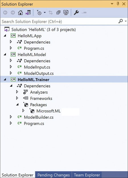
FIGURE 2-1 The skeleton of an ML.NET project in Visual Studio
Aside from the core references to the .NET framework of choice (whether 3.x or 5), the only additional piece you need to bring in is the Microsoft.ML NuGet package.
The package is not comprehensive, meaning that depending on what you intend to do, installing more packages might be necessary. However, the package is sufficient to get you started and enables you to experiment with the library. Let’s focus on the trainer application and see what it takes to interact with the ML.NET library.
The Pipeline Entry Point
The entry point in the ML.NET pipeline is the MLContext object. You use it in much the same way you use the Entity Framework DBContext object or the connection object to a database library. You need to have an instance of this class shared across the various objects that participate in the building of the model. A common practice employed in most tutorials—including the sample code generated by the aforementioned Model Builder wizard—is wrapping the model building workflow in a dedicated class, often just named ModelBuilder.
public static class ModelBuilder
{
    private static MLContext Context = new MLContext();

   // Main method
   public static void CreateModel(string inputDataFileName, string outputModelFileName)
   {
      // Load data

      // Build training pipeline

      // Train Model

      // QUICK evaluation of the model

      // Save the output model

   }
}
The instance of the MLContext class is global to the class methods, and the name of the files containing train data and the final output file are passed as arguments. The body of the CreateModel method (or whatever name you choose for it) develops around a few steps that involve more specific classes of the ML.NET library for activities such as data transformation, feature engineering, model selection, training, evaluation, and persistence.
Data Preparation
The ML.NET framework can read data from a variety of data sources (for example, a CSV-style text file, a binary file, or any IEnumerable-based object) and does that through the services of a few specialized loaders built around a specific interface—the IDataView interface, a flexible and efficient way of describing tabular data.
An IDataView-based loader works as a database cursor and supplies methods to navigate around the data set at any acceptable pace. It also provides an in-memory cache and methods to write the modified content back to disk. Here’s a quick example:
// Create the context for the pipeline
Context = new MLContext();

// Load data into the pipeline via the DataView object
var dataView = Context.Data.LoadFromTextFile<ModelInput>(INPUT_DATA_FILE);
The sample code loads training data from the specified file and manages it as a collection of ModelInput types. Needless to say, the ModelInput type is a custom class that reflects the rows of data loaded from the text file. The snippet below shows a sample ModelInput class. The LoadColumn attribute refers to the position of the CSV column to which the property binds.
public class ModelInput
{
  [LoadColumn(0)]
  public string Month { get; set; }

  [LoadColumn(1)]
  public float Sales { get; set; }
}
In the code, there’s an even more relevant point to emphasize. The code makes a key assumption that the loaded data is already in a format that is acceptable for machine learning operations. More often than not, instead, some transformation is necessary to perform on top of available data—the most important of which is that all data must be numeric because algorithms can only read numbers. Here’s a realistic scenario:
Your customer has a lot of data coming from a variety of data sources, whether timeline series, sparse Office documents, or database tables populated by online web frontends. In its raw format, the data—no matter the amount—might not be very usable. The appropriate format of the data depends on the desired result and the selected training algorithm. Therefore before mounting the final pipeline, a number of data transformation actions might be necessary, such as rendering data in columns, adding ad hoc feature columns, removing columns, aggregating and normalizing values, and adding density wherever possible. Depending on the context, these steps might be accomplished only once or every time the model is trained.
 Note
Note
At first sight, it might seem that integrating data processing in the pipeline is a waste of time and that there’s no value in doing it every time the model is built. More in general, instead, it is a matter of trade-off. We’re usually talking about large quantities of data, and processing it to some intermediate format may be expensive. On the other hand, if the gap between raw and cleaned data is not that big, transforming data on each build of the model can deliver tremendous flexibility because you can change the transformation parameters as is convenient. It’s a pure speed versus flexibility trade-off.
Trainers and Their Categorization
Training is the crucial phase of a machine learning pipeline. The training consists of picking an algorithm, setting in some way its configuration parameters, and running it repeatedly on a given (training) data set. The output of the training phase is the set of parameters that lead the algorithm to generate the best results. In the ML.NET jargon, the algorithm is called the trainer. More precisely, in ML.NET, a trainer is an algorithm plus a task. The same algorithm (say, L-BFGS) can be used for different tasks, such as regression or multiclass classification.
Table 2-1 lists some of the supported trainers grouped in a few tasks. We cover ML.NET tasks in more depth throughout the rest of the book and investigate their programming interface.
TABLE 2-1 ML.NET Tasks Related to Training
Task |
Description |
|---|---|
AnomalyDetection |
Aims at detecting unexpected or unusual events or behaviors compared to the received training |
BinaryClassification |
Aims at classifying data in one of two categories |
Clustering |
Aims at splitting data in a number of possibly correlated groups without knowing which aspects could possibly make data items related |
Forecasting |
Addresses forecasting problems |
MulticlassClassification |
Aims at classifying data in three or more categories |
Ranking |
Addresses ranking problems |
Regression |
Aims at predicting the value of a data item |
Figure 2-2 presents the list of ML.NET task objects as they show up through IntelliSense from the MLContext pipeline entry point.
)
FIGURE 2-2 The list of ML.NET task objects
Each of the task objects listed in Table 2-1 has a Trainers property that lists the predefined algorithms supported by the framework. For example, for a prediction task, a good algorithm is the Online Gradient Descent algorithm.
var dataProcessPipeline = mlContext.Transforms.Text.FeaturizeText(...);
var trainer = mlContext.Regression.Trainers.OnlineGradientDescent(...);
var trainingPipeline = dataProcessPipeline.Append(trainer);
The code snippet selects an instance of the algorithm and then appends it to the data processing pipeline at the end of which the compiled model will come out. This short code contains the essence of the whole ML.NET programming model. This is the way in which the whole pipeline is built step by step and then run.
It is also worth noting that ML.NET supports several specific algorithms for each predefined task. In particular, for the regression task the ML.NET framework also supports the “Poisson Regression” and the “Stochastic Dual Coordinate Ascent” algorithms, and many more can be added to the project at any time through new NuGet packages.
Once the pipeline is built and fully configured, it is ready to run on the provided data. In this regard, the pipeline is a sort of abstract workflow that processes data in a way comparable to how in .NET LINQ queryable objects work on collections and data sets.
Once trained, a model is nothing more than the serialization of a computation graph that represents some sort of mathematical expression or, in some cases, a decision tree. The exact details of the expression depend on the algorithm and to some extent, the nature of the problem’s category.
Model Training Executive Summary
Explaining the mechanics of model training is well beyond the scope of this book, which remains strictly focused on the ML.NET framework. However, at least a brief recap of what it means and how it works is in order. For an in-depth analysis, you can easily find online resources as well as books. In particular, you can take a look at our book Introducing Machine Learning (Microsoft Press, 2020), in which we mainly focus on the mathematics behind most problems and the algorithmic solutions discovered so far for each class.
Purpose of the Training Phase
Abstractly speaking, an algorithm is the sequence of steps that lead to the solution of a problem. In artificial intelligence, there are two main classes of problems: classification of entities and predictions. In each of these classes, we find several subclasses, such as ranking, forecasting, regression, anomaly detection, image and text analysis, and so forth.
In fact, the output of a machine learning pipeline is a software artifact made of an algorithm (or a chain of algorithms) whose parametric parts (settings and configurable elements) have been adjusted based on the provided training data. In other words, the output of a machine learning pipeline is the instance of an algorithm that, much like the instance of an object-oriented language class, has been initialized to hold a given configuration. The configuration to use for the instance of the algorithm is discovered during the training phase. The schema is outlined in Figure 2-3.
)
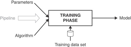
FIGURE 2-3 Overall schema of the training phase in a machine learning process
The Computation Graph
As mentioned, the model is a mathematical black-box—a computation graph—that takes input and computes an output. Input and output are lists of numbers, and in an object-oriented context—as in .NET—they are modeled using classes.
Figure 2-4 presents an abstract and concrete view of how a client application ultimately uses a trained model. Input data flows in, and the gears of the graph crunch numbers and produce a response for the application to deal with.
)
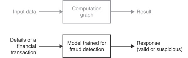
FIGURE 2-4 Overall schema of a trained model being used in production
For example, if you have a model trained to detect possible fraudulent transactions in a financial application, the graph in the model will be called to process a numeric representation of the transaction and produce some values that could be interpreted as to whether the transaction should be approved, denied, or just flagged for further investigation.
Performance of the Model
The term machine learning sounds fascinating, but it is not always fully representative of what really happens in a low-level ML framework such as ML.NET or Python’s scikit-learn. At this level, the training phase just iteratively processes records in the training data set to minimize an error function.
The function that produces values–the computation graph—is defined by the selected algorithm.
The error function is yet another element added to the processing pipeline and also depends, to some extent, on the selected algorithm.
The error function measures the distance between values produced by the graph on testing data and expected data embedded in the training data set.
The graph enters the training phase with a default configuration that is updated if the measured error is too large for the desired goal.
When a good compromise between speed and accuracy is reached, the training ends, and the current configuration of the graph is frozen and serialized for production.
The whole process develops iteratively in the training phase within the ML.NET framework. The steps are summarized in Figure 2-5.
)
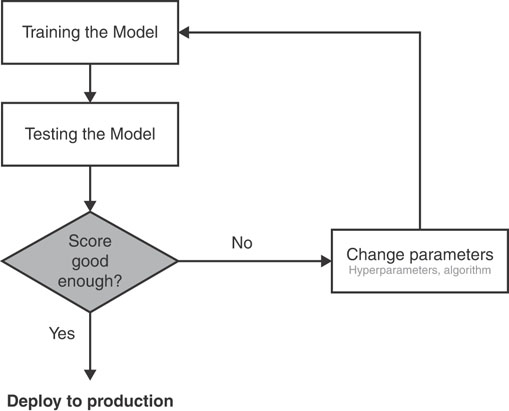
FIGURE 2-5 The generation of an ML model
It should be noted that the evaluation phase depicted here happens within the ML.NET framework and, more in general, within the boundaries of the ML framework of choice. The actual performance evaluated is obtainable on training data with a given set of algorithm parameters (referred to as hyperparameters) and internally computed coefficients.
This is not the same as measuring the performance of the model in production. At this stage, you only measure how good the model is at work on sample data. However, sample data is only expected to be a realistic snapshot of data the model will face once deployed to production. A more crucial evaluation phase will take place later and might even take to rebuilding the model based on different hyperparameters and—why not?—a different algorithm.
In ML.NET, the quality of the model during the training phase is measured using special components called evaluators.
A Look at Evaluators
An evaluator is a component that implements a given metric. Evaluation metrics are specific to the class of the algorithm and, in ML.NET, to the ongoing ML task. A good introduction on which evaluator is deemed appropriate for each ML.NET task can be found at
https://docs.microsoft.com/en-us/dotnet/machine-learning/resources/metrics.
A more in-depth discussion about the mathematical reasons that make each metric qualified for a given task can be found in the aforementioned book Introducing Machine Learning.
For example, for a prediction problem such as estimating the cost of a taxi ride (and in general for regression and ranking/recommendation problems), a key metric to consider is Squared Loss, also known as Mean Squared Error (MSE). This metric works by measuring how close a regression line is to test expected values. For each input test value, the evaluator takes the distance between the computed and the expected response, squares it, and then calculates the mean. The squaring is applied to increase the relevance of larger differences.
Interestingly, Model Builder, which is embedded in Visual Studio, does some of the work for you. It first lets you choose the class of the problem (the ML task) and indicate the training data set. Based on that, it automatically selects a few matching algorithms, trains them, and measures the performance according to automatically selected metrics. Then it makes a final call and recommends how you should start coding your machine learning solution.
In general, there are a few things that could possibly go bad in a machine learning project:
The selected algorithm (or algorithm hyperparameters) might not be the most appropriate to explore the given data set.
The original data set needs more (or less) column transformation.
The original data set is too small for the intended purpose.
As an example, Table 2-2 summarizes the scores of various algorithms selected by Model Builder for a prediction (regression) task.
TABLE 2-2 Multiple algorithms (and scores) for a sample regression task
Algorithm |
Squared Loss |
Absolute Loss |
RSquared |
RMS Loss |
|---|---|---|---|---|
LightGbmRegression |
4.49 |
0.38 |
0.9513 |
2.12 |
FastTreeTweedieRegression |
4.70 |
0.44 |
0.9491 |
2.17 |
FastTreeRegression |
4.83 |
0.41 |
0.9486 |
2.19 |
SdcaRegression |
10.52 |
0.87 |
0.8845 |
3.27 |
After a test run of Model Builder, it shows that all featured algorithms ended up with good marks, but Model Builder ranked them in the order shown, thus suggesting we use the LightGbmRegression algorithm based on the evidence provided by metrics. Look in particular at the Squared Loss column. The score is acceptably good for the first three ranked algorithms and significantly worse for SdcaRegression. On the other hand, SdcaRegression is much faster to train. The golden rule of machine learning is that everything is a trade-off.
Note
Another aspect to consider is that once the model goes to production—even with the best metrics—there might still be chances that things go wrong and the predictions are not in line with business expectations. When this happens, the odds are that an inadequate set of data rows was used for training. Inadequate, at least, in comparison to the real data the model was called to manage in production.