Objective group 2. Manage data cells and ranges

Objective 2.2: Format cells and ranges

Merge and unmerge cells

Worksheets that involve data at multiple hierarchical levels often use horizontal and vertical merged cells to clearly delineate relationships. Excel provides the following three merge options:

• Merge & Center This option merges the cells across the selected rows and columns and centers the data from the first selected cell in the merged cell.

• Merge Across This option creates a separate merged cell for each row in the selection area and maintains default alignment for the data type of the first cell of each row of the merged cells.

• Merge Cells This option merges the cells across the selected rows and columns and maintains default alignment for the data type of the first cell of the merged cells.

In the case of Merge & Center and Merge Cells, data in selected cells other than the first is deleted. In the case of Merge Across, data in selected cells other than the first cell of each row is deleted.

To merge selected cells

• ➜ On the Home tab, in the Alignment group, click the Merge & Center button to center and bottom-align the entry from the first cell.

• ➜ On the Home tab, in the Alignment group, display the Merge & Center list, and then click Merge Across to create a separate merged cell on each selected row, maintaining the horizontal alignment of the data type in the first cell of each row.

• ➜ On the Home tab, in the Alignment group, display the Merge & Center list, and then click Merge Cells to merge the entire selection, maintaining the horizontal alignment of the data type in the first cell.

To unmerge selected cells

• ➜ On the Home tab, in the Alignment group, click the Merge & Center button to deselect it.

Modify cell alignment, orientation, and indentation

Structural formatting can be applied to a cell, a row, a column, or the entire worksheet. However, some kinds of formatting can detract from the readability of a worksheet if they are applied haphazardly.

The formatting you might typically apply to a row or column includes the following:

• Alignment You can specify a horizontal alignment (Left, Center, Right, Fill, Justify, Center Across Selection, and Distributed) and vertical alignment (Top, Center, Bottom, Justify, or Distributed) of a cell’s contents. The defaults are Left and Top, but in many cases another alignment will be more appropriate.

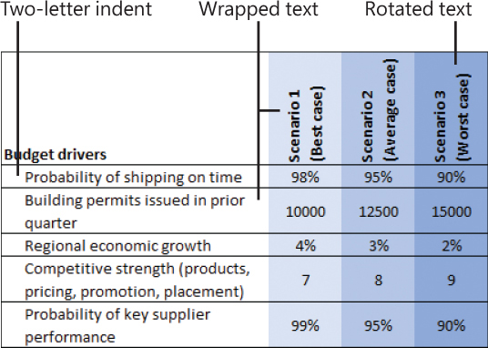
• Orientation By default, entries are horizontal and read from left to right. You can rotate entries for special effect or to allow you to display more information on the screen or a printed page. This capability is particularly useful when you have long column headings above columns of short entries.

• Indentation You can specify an indent distance from the left or right side when you choose those horizontal alignments, or from both sides when you choose a distributed horizontal alignment. A common reason for indenting cells is to create a list of subitems without using a second column.

To open the Format Cells dialog box to the most recently used tab

• ➜ On the Home tab, click the Font dialog box launcher.

• ➜ Press Ctrl+1.

To align entries within selected cells

• ➜ On the Home tab, in the Alignment group, click the Align Left, Center, or Align Right button to specify horizontal alignment, or click the Top Align, Middle Align, or Bottom Align button to specify vertical alignment.

• ➜ On the Home tab, click the Alignment dialog box launcher. On the Alignment tab of the Format Cells dialog box, in the Horizontal and Vertical lists, click the cell alignment you want.

  

  Configure text alignment, indents, orientation, and wrapping options at one time from the Format Cells dialog box

To change the orientation of the text in selected cells

1. On the Home tab, in the Alignment group, click the Orientation button to display the Alignment tab of the Format Cells dialog box.

2. In the Orientation area, do either of the following:

   • Drag the red diamond to the angle you want.

   • In the Degrees list, click the angle you want.

   The Text preview changes to display the effect of your selection.

3. In the Format Cells dialog box, click OK.

To indent the content of selected cells

1. On the Home tab, click the Alignment dialog box launcher.

2. On the Alignment tab of the Format Cells dialog box, in the Text alignment section, do the following:

   1. In the Horizontal list, select Left (Indent), Right (Indent), or Distributed (Indent).

   2. In the Indent box, enter or select the number of characters by which you want to indent the text. Then click OK.

3. In the Format Cells dialog box, click OK.

Wrap text within cells

By default, Excel does not wrap text in a cell. Instead, it allows the entry to overflow into the surrounding cells (to the right from a left-aligned cell, to the left from a right-aligned cell, and to both sides from a center-aligned cell) if those cells are empty, or it hides the part that won’t fit if the surrounding cells contain content. To make the entire entry visible, you can allow the cell entry to wrap to multiple lines.

To wrap long entries in selected cells

• ➜ On the Home tab, in the Alignment group, click the Wrap Text button.

Apply cell formats and styles

By default, the font used for text in a new Excel worksheet is 11-point Calibri, but you can use the same techniques you would use in any Office 2019 program to change the font and the following font attributes:

• Size

• Style

• Color

• Underline

As a certification candidate, you should be very familiar with methods of applying character formatting from the Font group on the Home tab, from the Mini Toolbar, and from the Font, Border, and Fill tabs of the Format Cells dialog box.

Cell Styles are preconfigured sets of cell formats, some tied to the workbook theme colors and some with implied meanings. You can standardize formatting throughout workbooks by applying cell styles to content.

To apply cell formatting from the Format Cells dialog box to selected cells

1. On the Home tab, click the Font dialog box launcher.

2. In the Format Cells dialog box, on the Font, Border, and Fill tabs, select the formatting you want to apply to the cell and its content. Then click OK.

To apply a cell style to a selected cell

1. On the Home tab, in the Styles group, click the Cell Styles button.

2. In the Cell Styles gallery, click the style you want.

Apply number formats

By default, all the cells in a new worksheet are assigned the General number format. When setting up or populating a worksheet, you assign to cells the number format that is most appropriate for the type of information they contain. The format determines not only how the information looks, but also how Excel can work with it.

You can assign a number format to a cell before or after you enter a number in it. You can also just start typing and have Excel intuit the format from what you type. (For example, if you enter 9/15, Excel makes the educated guess that you’re entering a date and applies the default date format d-mmm, resulting in 15-Sep.) When you allow Excel to assign a number format, or you choose a format from the Number Format list in the Number group on the Home tab, Excel uses the default settings for that format. You can change the currency symbol and the number of decimal places shown directly from the Number group. You can change many other settings (such as changing the format of calendar dates from 15-Sep to September 15, 2019) from the Format Cells dialog box.

When you apply the Percentage number format to a cell, the cell displays the percentage equivalent of the number. For example, the number 1 is shown as 100%, the number 5 as 500%, or the number 0.25 as 25%.

To apply a default number format to selected cells

• ➜ On the Home tab, in the Number group, display the Number Format list, and then click a format.

To display the percentage equivalent of a number

1. Select the cell or cells you want to format.

2. Do either of the following:

   • On the Home tab, in the Number group, click the Percent Style button.

   • Press Ctrl+Shift+%.

To display a number as currency

1. Select the cell or cells you want to format.

2. On the Home tab, in the Number group, do one of the following:

   • To format the number in the default currency, click the Accounting Number Format button (labeled with the default currency symbol).

   • To format the number in dollars, pounds, euros, yen, or Swiss francs, click the Accounting Number Format arrow, and then click the currency you want.

   • To format the number in a currency other than those listed, click the Accounting Number Format arrow, and then click More Accounting Formats to display the Accounting options.

     

     You can choose from hundreds of currencies

3. In the Format Cells dialog box, do the following, and then click OK:

   1. In the Symbol list, select the currency symbol you want to display.

   2. In the Decimal places box, enter or select the number of decimal places you want to display.

To display more or fewer decimal places for numbers

1. Select the cell or cells you want to format.

2. On the Home tab, in the Number group, do either of the following:

   • To display more decimal places, click the Increase Decimal button.

   • To display fewer (or no) decimal places, click the Decrease Decimal button.

To apply a number format with settings other than the default

1. Select the cell or cells you want to format.

2. On the Home tab, click the Number dialog box launcher.

3. On the Number tab of the Format Cells dialog box, select the type of number in the Category list.

4. Configure the settings that are specific to the number category, and then click OK.

Reapply existing formatting

If you apply a series of formats to one or more cells—for example, if you format cell content as 14-point, bold, centered, red text—and then want to apply the same combination of formatting to other cells, you can copy the formatting. You can use the fill functionality to copy formatting to adjacent content, or use the Format Painter to copy formatting anywhere. When using the Format Painter, you first copy existing formatting from one or more cells, and then paste the formatting to other cells. You can use the Format Painter to paste copied formatting only once or to remain active until you turn it off.

To copy existing formatting to other cells

1. Select the cell that has the formatting you want to copy.

2. On the Mini Toolbar or in the Clipboard group on the Home tab, click the Format Painter button once if you want to apply the copied formatting only once, or twice if you want to apply the copied formatting multiple times.

3. With the paintbrush-shaped cursor, click or select the cell or cells to which you want to apply the copied formatting.

4. If you clicked the Format Painter button twice, click or select additional cells you want to format. Then click the Format Painter button again, or press the Esc key, to turn off the Format Painter.

To fill formatting to adjacent cells

1. Select the cell that has the formatting you want to copy.

2. Drag the fill handle up, down, to the left, or to the right to encompass the cells you want to format.

3. On the Auto Fill Options menu, click Fill Formatting Only.