Manage and Format Data in Excel

Objective 2.2: Format and validate data

Create custom number formats

One of the best ways to improve the readability of your worksheets is to display your data in a format that is logical, consistent, and straightforward. Formatting currency amounts with leading dollar signs, percentages with trailing percent signs, and large numbers with commas are a few of the ways you can improve your spreadsheet style. However, you can use Excel to go beyond these built-in formats to create custom number and date formats with which you can display your worksheet values exactly as you want them to be seen.

Excel’s built-in numeric formats give you a great deal of control over how your numbers are displayed, but they have their limitations. For example, there is no built-in format you can use to display a different currency symbol, such as the Euro symbol (€), or to display temperatures using, say, the degree symbol (°).

To overcome these limitations, you need to create your own custom numeric formats. You can do this either by editing an existing format or by entering your own format from scratch. The formatting syntax and symbols are explained in detail later in this section.

Every Excel numeric format, whether built-in or customized, has the following syntax:

positive format;negative format;zero format;text format

The four parts, separated by semicolons, determine how various numbers are presented. The first part defines how a positive number is displayed, the second part defines how a negative number is displayed, the third part defines how zero is displayed, and the fourth part defines how text is displayed. If you leave out one or more of these parts, numbers are controlled as shown in the following table.

Number of parts used	Format syntax
Three	positive format;negative format;zero format
Two	positive and zero format;negative format
One	positive, negative, and zero format

The following table lists the special symbols you use to define each of these parts.

Symbol	Description
#	Holds a place for a digit and displays the digit exactly as typed. Displays nothing if no number is entered. For example, if a cell’s custom format is ### and you enter 25 in the cell, Excel displays 25.
0	Holds a place for a digit and displays the digit exactly as typed. Displays zero if no number is entered. For example, if a cell’s custom format is 000 and you enter 25 in the cell, Excel displays 025.
?	Holds a place for a digit and displays the digit exactly as typed. Displays a space if no number is entered. For example, if a cell’s custom format is 0??? and you enter 25 in the cell, Excel displays 0 25.
. (period)	Sets the location of the decimal point. For example, if a cell’s custom format is #.#0 and you enter 34.5 in the cell, Excel displays 34.50.
, (comma)	Sets the location of the thousands separator. Marks only the location of the first thousand. For example, if a cell’s custom format is #,### and you enter 12345 in the cell, Excel displays 12,345.
%	Multiplies the number by 100 (for display only) and adds the percent (%) character. For example, if a cell’s custom format is #% and you enter .75 in the cell, Excel displays 75%.
E+ e+ E- e-	Displays the number in scientific format. E- and e- place a minus sign in the exponent; E+ and e+ place a plus sign in the exponent. For example, if a cell’s custom format is 0.00E+00 and you enter 123456789 in the cell, Excel displays 1.23E+08. Similarly, if a cell’s custom format is 0.0E-00 and you enter 0.0000012 in the cell, Excel displays 1.2E-06.
/ (slash)	Sets the location of the fraction separator. For example, if a cell’s custom format is 0/0 and you enter .75 in the cell, Excel displays 3/4.
$ ( ) : - + <space>	Displays the character. For example, if a cell’s custom format is $##0.00 and you enter 123.5 in the cell, Excel displays $123.50.
*	Repeats whatever character immediately follows the asterisk until the cell is full. Doesn’t replace other symbols or numbers. For example, you can create a dot trailer in a cell by adding *. to the format. So if the custom format is #*. and you enter 123 in the cell, Excel displays 123............ (where the dots continue until the cell is filled).
_ (underscore)	Inserts a blank space the width of whatever character follows the underscore, which can often help you to align your numbers. For example, the custom format _(#.00 inserts a blank space the width of the opening parenthesis at the beginning of the displayed value.
\ (backslash)	Inserts the character that follows the backslash. See the next item for an example. In general, you need to use the backslash only for reserved characters (such as # or @) or for the following letters: B, D, E, G, H, M, N, S, and Y. (For all other letters, if you just enter a single character by itself, Excel will display that character.) For example, if a cell’s custom format is #.##\M and you enter 1.23 in the cell, Excel displays 1.23M.
“text”	Inserts the text that appears within the quotation marks. For example, if a cell’s custom format is “Part “\#00-0000 and you enter 123456 in the cell, Excel displays Part #12-3456.
@	Displays the cell’s text. For example, if a cell’s custom format is @” entry” and you enter credit in the cell, Excel displays credit entry.
[color]	Displays the cell contents in the specified color. For example, if the cell’s custom format is [green]0.00; [red]0.00, Excel displays positive cell values in green and negative cell values in red. The predefined color values you can use are black, white, red, green, blue, yellow, magenta, and cyan, and the color codes color1 through color565.

Although the built-in date and time formats of Excel are fine for most purposes, you might need to create your own custom formats. For example, you might want to display the day of the week (for example, “Friday”). Custom date and time formats generally are simpler to create than custom numeric formats. There are fewer formatting symbols, and you usually don’t need to specify different formats for different conditions. The following table lists the date and time formatting symbols.

Symbol	Description
Date Formats
d	Day number without a leading zero (1 to 31)
dd	Day number with a leading zero (01 to 31)
ddd	Three-letter day abbreviation (Mon, for example)
dddd	Full day name (Monday, for example)
m	Month number without a leading zero (1 to 12)
mm	Month number with a leading zero (01 to 12)
mmm	Three-letter month abbreviation (Aug, for example)
mmmm	Full month name (August, for example)
yy	Two-digit year (00 to 99)
yyyy	Full year (1900 to 2078)
h	Hour without a leading zero (0 to 24)
hh	Hour with a leading zero (00 to 24)
m	Minute without a leading zero (0 to 59)
mm	Minute with a leading zero (00 to 59)
s	Second without a leading zero (0 to 59)
ss	Second with a leading zero (00 to 59)
AM/PM, am/pm, A/P	Displays the time using a 12-hour clock
/ : . —	Symbols used to separate parts of dates or times
[color]	Displays the date or time in the color specified

The best way to become familiar with custom formats is to try your own experiments. Excel stores each format that you try. If you find that your list of custom formats is getting a bit unwieldy or that it’s cluttered with unused formats, you can delete those formats.

To open the Format Cells dialog box, do one of the following:

• ➜ On the Home tab, in the Cells group, click Format, then click Format Cells.

• ➜ Right-click the cell or range, then click Format Cells.

• ➜ Press Ctrl+1.

To create and apply a custom number format

1. Select the cell or range of cells you want the new format to apply to.

2. Open the Format Cells dialog box.

3. On the Number tab, in the Category list, click Custom.

4. To base the custom number format on an existing format, click the base format in the Type list.

5. Edit or enter the symbols that define the number format.

   

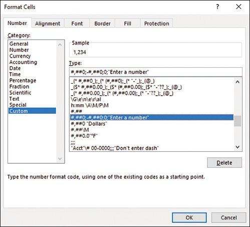
   Define custom number formats in the Type box.

6. When you are done, click OK to return to the worksheet.

To delete custom number formats

1. Display the Number tab of the Format Cells dialog box.

2. In the Category list, click Custom.

3. In the Type list, click the format you want to remove.

   TIP

   You can delete only custom formats; you can’t delete built-in formats.

4. Click Delete to remove the format from the list.

5. Click OK to close the Format Cells dialog box and return to the worksheet.

Configure data validation

Formulas are only as good as the data they’re given. For basic data entry errors (for example, entering the wrong date or transposing a number’s digits), there’s not much you can do other than exhort yourself or the people who use your worksheets to enter data carefully. Fortunately, you have a bit more control when it comes to preventing the entry of improper data such as data that is the wrong type (for example, entering text in a cell that requires a number) or data that falls outside of an allowable range (for example, entering 200 in a cell that requires a number between 1 and 100).

You can prevent these kinds of improper entries, to a certain extent, by adding comments that describe what is allowable inside a particular cell. However, this requires other people to both read and act on the comment text. You can also use custom numeric formatting to “format” a cell with an error message if the wrong type of data is entered. This is useful, but it works only for certain kinds of input errors.

The best solution for preventing data entry errors is to use the data-validation feature of Excel. With data validation, you create rules that specify exactly what kind of data can be entered and in what range that data can fall. You can also specify pop-up input messages that appear when a cell is selected and error messages that appear when data is entered improperly.

You configure data-validation rules on the Settings tab of the Data Validation dialog box. The following validation types are available:

• Any Value Allows any value in the range (that is, it removes any previously applied validation rule). If you’re removing an existing rule, be sure to also clear the input message, if any.

• Whole Number Allows only whole numbers (integers). You use the Data list to select a comparison operator (such as Between, Equal To, or Less Than) and then enter the specific criteria. For example, if you click the Between option, you must enter Minimum and Maximum values.

• Decimal Allows decimal numbers or whole numbers. You use the Data list to select a comparison operator and then enter the specific numeric criteria.

• List Allows only values specified in a list. You specify the allowable values in the Source box on the Settings tab of the Data Validation dialog box, either by specifying a range on the same sheet or a range name on any sheet that contains the list of allowable values (preceding the range or range name with an equal sign) or by entering the allowable values directly into the Source box (separated by commas). You have the option of allowing the user to select from the allowable values by using a list.

• Date Allows only dates. (If the user includes a time value, the entry is invalid.) You use the Data list to select a comparison operator and then enter the specific date criteria (such as a Start date and an End date).

• Time Allows only times. (If the user includes a date value, the entry is invalid.) You use the Data list to select a comparison operator and then enter the specific time criteria (such as a Start time and an End time).

• Text Length Allows only alphanumeric strings of a specified length. You use the Data list to select a comparison operator and then enter the specific length criteria (such as Minimum and Maximum lengths).

• Custom You can use this option to enter a formula that specifies the validation criteria. You can either enter the formula directly in the Formula box on the Settings tab of the Data Validation dialog box (again preceding the formula with an equal sign) or enter a reference to a cell that contains the formula. For example, if you’re restricting cell A2 and you want to be sure the entered value is not the same as what’s in cell A1, you would enter the formula =A2<>A1.

  

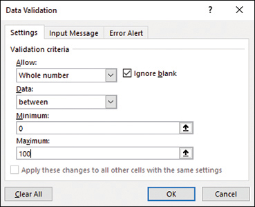
  On the Settings tab of the Data Validation dialog box, set up the criteria for your validation rule.

To configure data validation for a cell or range

1. Select the cell or range to which you want to apply the data-validation rule.

2. On the Data tab, in the Data Tools group, click Data Validation to open the Data Validation dialog box.

3. On the Settings tab, in the Allow list, click one of the validation types.

4. Enter the validation criteria you require.

5. To allow blank entries, either in the cell itself or in other cells specified as part of the validation settings, leave the Ignore blank check box selected. If you clear this check box, Excel treats blank entries as zero and applies the validation rule accordingly.

6. If the range had an existing validation rule that also applied to other cells, you can apply the new rule to those other cells by selecting the Apply these changes to all other cells with the same settings check box.

7. If you want a message to appear when the user selects the restricted cell or any cell within the restricted range, on the Input Message tab, do the following:

   Verify that the Show input message when cell is selected check box is selected.

   In the Title box, enter a title for the message.

   In the Input message box, enter the message that you want Excel to display. For example, you could use the message to give the user information about the type and range of allowable values.

   

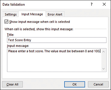
   You can configure an input message to appear when a workbook user selects the cell.

8. If you want a dialog box to appear when the user enters invalid data, click the Error Alert tab, then do the following:

   Select the Show error alert after invalid data is entered check box.

   In the Style list, click the error style you want: Stop, Warning, or Information.

   In the Title box, enter a title for the message.

   In the Error message box, enter the message that you want Excel to display.

   IMPORTANT

   Only the Stop style prevents users from entering invalid data.

   

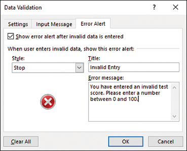
   You can configure an error alert to appear when a workbook user enters an invalid entry.

9. Click OK to apply the data-validation rule.

Group and ungroup data

You can control a worksheet range display by grouping the data based on the worksheet formulas and data. Grouping the data creates a worksheet outline, which you can use to “collapse” sections of the sheet to display only summary cells, or to “expand” hidden sections to show the underlying detail.

Not all worksheets can be grouped, so you need to make sure your worksheet is a candidate for outlining. First, the worksheet must contain formulas that reference cells or ranges directly adjacent to the formula cell. Worksheets with SUM functions that subtotal cells above or to the left are particularly good candidates for outlining.

Second, there must be a consistent pattern to the direction of the formula references. For example, a worksheet with formulas that always reference cells above or to the left can be outlined. Excel will not outline a worksheet with, say, SUM functions that reference ranges above and below a formula cell.

If your worksheet meets these criteria, then you can use Excel’s Auto Outline command to automatically group the worksheet data. Otherwise, you can group data manually.

When Excel creates an outline, it divides your worksheet into a hierarchy of levels. These levels range from the worksheet detail (the lowest level) to the grand totals (the highest level). Excel outlines can handle up to eight levels of data. In the Budget worksheet shown below, for example, Excel created three levels for both the column and the row data:

• In the columns, the monthly figures are the details, so they’re the lowest level (level 3). The quarterly totals are the first summary data, so they’re the next level (level 2). Finally, the grand totals (not shown) are the highest level (level 1).

• In the rows, the individual sales and expense items are the details (level 3). The sales and expenses subtotals are the next level (level 2). The Gross Profit row is the highest level (level 1).

To help you work with your outlines, Excel adds the following tools to your worksheet:

• Level bars—These bars indicate the data included in the current level. Click a bar to hide the rows or columns marked by a bar.

• Collapse symbol—Click this symbol to hide (or collapse) the rows or columns marked by the attached level bar.

• Expand symbol—When you collapse a level, the collapse symbol changes to an expand symbol (+). Click this symbol to display (or expand) the hidden rows or columns.

• Level symbols—These symbols tell you which level each level bar is on. Click a level symbol to display all the detail data for that level.

  TIP

  To toggle the outline symbols on and off, press Ctrl+8.

To group a worksheet using Auto Outline

• ➜ On the Data tab, in the Outline group, click Group, then click Auto Outline.

To group data manually

• ➜ Select the rows or columns you want to group, then on the Data tab, in the Outline group, click Group, then click Group.

Or,

1. Select a cell in each row or column you want to group.

2. On the Data tab, in the Outline group, click Group, then click Group. Excel asks whether you want to group rows or columns.

3. Select either Rows or Columns, as appropriate for your data, then click OK.

   

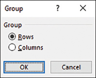
   When you group data manually, Excel needs to know whether you’re grouping rows or columns.

To remove an outline from a worksheet

• ➜ On the Data tab, in the Outline group, click Ungroup, then click Clear Outline.

To ungroup data

• ➜ Select the rows or columns you want to ungroup, then on the Data tab, in the Outline group, click Ungroup, then click Ungroup.

Or,

1. Select a cell in each row or column you want to ungroup.

2. On the Data tab, in the Outline group, click Ungroup, then click Ungroup. Excel asks whether you want to ungroup rows or columns.

3. Select either Rows or Columns, as appropriate for your data, then click OK.

Calculate data by inserting subtotals and totals

Although you can use formulas and worksheet functions to summarize your data in various ways—including sums, averages, counts, maximums, and minimums—if you’re in a hurry, or if you just need a quick summary of your data, you can get Excel to do the work for you. The secret here is a feature called automatic subtotals, which are formulas that Excel adds to a worksheet automatically.

Excel sets up automatic subtotals based on data groupings in a selected field. For example, if you ask for subtotals based on the Customer field, Excel runs down the Customer column and creates a new subtotal each time the name changes. To get useful summaries, you should sort the range on the field containing the data groupings you’re interested in.

Note that in the phrase automatic subtotals, the word subtotals is misleading because it implies that you can only summarize your data with totals. However, you can also count the values (all the values or just the numeric values), calculate the average of the values, determine the maximum or minimum value, and calculate the product of the values. For statistical analysis, you can also calculate the standard deviation and variance, both of a sample and of a population.

To insert subtotals and totals

1. Select a cell within the range you want to subtotal.

2. On the Data tab, in the Outline group, click Subtotal to open the Subtotal dialog box.

3. Use the At each change in list to select the column you want to use to group the subtotals.

4. In the Use function list, select Sum.

5. In the Add subtotal to list, select the check box for the column you want to summarize.

   

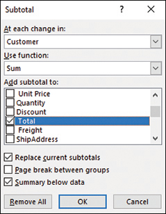
   Use the Subtotal dialog box to apply subtotals to a range.

6. Click OK. Excel calculates the subtotals and adds them to the range and also adds a Grand Total row to the bottom of the range. Excel also adds outline symbols to the range.

To change the summary calculation

• ➜ In step 4 from the previous section, in the Use function list, select the function you want to use, such as Count, Average, Max, or Min.

Remove duplicate records

You can make your Excel data more accurate for analysis by removing duplicate records. Duplicate records throw off calculations by including the same data two or more times. To prevent this, you should delete duplicate records. Rather than looking for duplicates manually, you can use the Remove Duplicates command, which quickly finds and removes duplicates in even the largest ranges or tables.

Before you use the Remove Duplicates command, you must decide what defines a duplicate record in your data. You have two choices:

• Two records are duplicates if, for every column in the range or table, the records contain identical values.

• Two records are duplicates if, for only certain columns in the range or table, the records contain identical values.

To remove duplicate records

1. Click a cell inside the range or table.

2. On the Data tab, in the Data Tools group, click Remove Duplicates to open the Remove Duplicates dialog box.

3. If your range doesn’t have column headers, clear the My data has headers check box.

4. Select the check box beside each field that you want Excel to check for duplicate values.

   TIP

   If your range or table has many fields, you may want Excel to use only one or two of those fields to look for duplicate records. Rather than clearing all the other check boxes manually, first click Unselect All in the Remove Duplicates dialog box to clear all the check boxes. You can then click to select just the check boxes you want Excel to use.

   

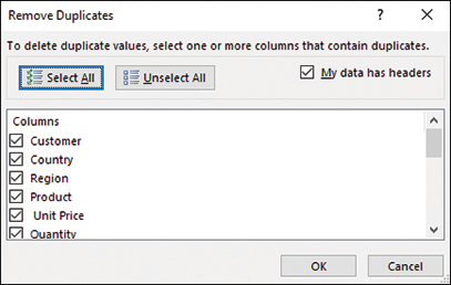
   Use the Remove Duplicates dialog box to specify which columns must contain identical data for the records to be considered duplicates.

   IMPORTANT

   Excel does not give you a chance to confirm the deletion of the duplicate records, so be sure you want to do this before proceeding.

5. Click OK. Excel deletes any duplicate records that it finds and then displays a dialog box telling you the number of duplicate records that it deleted.

   

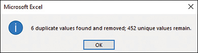
   Excel tells you how many duplicate records it deleted and how many unique records remain in the range or table.

6. Click OK.