Mapping Problems and Algorithms with Machine Learning

When I consider what people generally want in calculating, I found that it always is a number.

—Muḥammad ibn Mūsā al-Khwārizmī

Persian mathematician of eighth century whose name originated the word algorithm

More often than not, the user experience produced by machine learning looks like magic to users. At the end of the day, though, machine learning is only a new flavor of software—a new specialty much like web or database development—and a flavor of software that today is a real breakthrough.

A breakthrough technology is any technology that enables people to do things that weren’t possible before. Behind the apparent magic of final effects, however, there is a series of cumbersome tasks and, more than everything else, there’s a series of sequential and interconnected decisions along the way that are hard to make and time consuming. In a nutshell, they are critical decisions for the success of the solution.

This chapter has two purposes. First, it identifies the classes of problems that machine learning can realistically address and the algorithms known to be appropriate for each class. Second, it introduces a relatively new approach—automated machine learning or AutoML for short—that can automate the selection of the best machine learning pipeline for a given problem and a given dataset.

In this chapter, we’ll describe classes of problems and classes of algorithms. We’ll focus on the building blocks of a learning pipeline in the next chapter.

Fundamental Problems

As you saw in Chapter 2, “Intelligent Software,” the whole area of machine-based learning can be split into supervised and unsupervised learning. It’s an abstract partition of the space of algorithms, and the main discriminant for being supervised or unsupervised is whether or not the initial dataset includes valid answers. Put another way, we can reduce automated learning into the union of two learning approaches—learning by example (supervised) and learning by discovery (unsupervised).

Under these two forms of learning, we can identify a number of general problems and for each a number of general algorithms. This layout is reflected in the organization of any machine learning software development library you can find out there and use—whether it’s based on Python, Java, or .NET.

Classifying Objects

The classification problem is about identifying the category an object belongs to. In this context, an object is a data item and is fully represented by an array of values (known as features). Each value refers to a measurable property that makes sense to consider in the scenario under analysis. It is key to note that classification can predict values only in a discrete, categorical set.

Variations of the Problem

The actual rules that govern the object-to-category mapping process lead to slightly different variations of the classification problem and subsequently different implementation tasks.

• Binary Classification. The algorithm has to assign the processed object to one of only two possible categories. An example is deciding whether, based on a battery of tests for a particular disease, a patient should be placed in the “disease” or “no-disease” group.

• Multiclass Classification. The algorithm has to assign the processed object to one of many possible categories. Each object can be assigned to one and only one category. For example, classifying the competency of a candidate, it can be any of poor/sufficient/good/great but not any two at the same time.

• Multilabel Classification. The algorithm is expected to provide an array of categories (or labels) that the object belongs to. An example is how to classify a blog post. It can be about sports, technology, and perhaps politics at the same time.

• Anomaly Detection. The algorithm aims to spot objects in the dataset whose property values are significantly different from the values of the majority of other objects. Those anomalies are also often referred to as outliers.

Commonly Used Algorithms

At the highest level of abstraction, classification is the process of predicting the group to which a given data item belongs. In stricter math terms, a classification algorithm is a function that maps input variables to discrete output variables. (See Figure 3-1.)

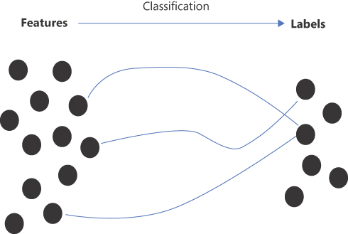
Figure 3-1 A graphical representation of a classification function

The classes of algorithms most commonly used for classification problems are as follows:

• Decision Tree. A decision tree is a tailor-made binary tree that implements a sequence of rules to be progressively applied to each input object. Each leaf of the tree represents one of the possible output categories. Along the way, the input object is routed downward through the levels of the tree based on rules set at each node. Each rule is based on a possible value of one of the features. In other words, at each step, the key feature value of the input object (say, Age) is checked against the set value (say, 40), and the visit proceeds in the subtree that applies (say, less than or greater than or equal to 40). The number of nodes and the feature/value rules implemented are determined during the training of the algorithm.

• Random Forest. This is a more specialized version of the decision tree algorithm. Instead of a single tree, the algorithm uses a forest of simpler trees trained differently and then provides a response that is some average of all the responses obtained.

• Support Vector Machine. Conceptually, this algorithm represents the input values as points in an n-dimensional space and looks for a sufficiently wide gap between points. In two dimensions, you can imagine the algorithm looking for a curve that cuts the plane in two, leaving as much space as possible along the margin. In three dimensions, you can think of a plane that cuts the space in two.

• Naïve Bayes. This algorithm works by computing the probability that a given object, given its values, may fall in one of the predefined categories. The algorithm is based on Bayes’ theorem, which describes the likelihood of an event given some related conditions.

• Logistic Regression. This algorithm calculates the probability of an object falling in a given category given its properties. The algorithm uses a sigmoid (logistic) function that, for its mathematical nature, lends itself well to be optimized to calculate a probability very close to 1 (or very close to 0). For this reason, the algorithm works well in either/or scenarios, and so it is mostly used in binary classification.

The preceding list is not exhaustive but includes the most-used classes of algorithms battle-tested for classification problems.

Common Problems Addressed by Classification

A number of real-life problems can be modeled as classification problems, whether binary, multiclass, or multilabel. Again, the following list can’t and won’t be exhaustive, but it is enough to give a clue about where to look when a concrete business issue surfaces:

• Spam and customer churn detection

• Data ranking and sentiment analysis

• Early diagnosis of a disease from medical images

• A recommender system built for customers

• News tagging

• Fraud or fault detection

Spam detection can be seen as a binary classification problem: an email is spam or is not. The same can be said for early diagnosis solutions although in this case the nature of the input data—images instead of records of data—requires a more sophisticated pipeline and probably would be solved using a neural network rather than any of the algorithms described earlier. Customer churn detection and sentiment analysis are multiclass problems, whereas news tagging and recommenders are multilabel problems. Finally, fraud or fault detection can be catalogued as an anomaly detection problem.

Predicting Results

Many would associate artificial intelligence with the ability to make smart predictions about future events. In spite of appearances, prediction is not magic but the result of a few statistical techniques, the most relevant of which is regression analysis. Regression measures the strength of a relationship set between one output variable and a series of input variables.

Regression is a supervised technique and is used to predict a continuous value (as opposed to discrete categorical values of classification).

Variations of the Problem

Regression is about finding a mathematical function that captures the relationship between input and output values. What kind of function? Different formulations of the regression function lead to different variations of the regression problem. Here are some macro areas:

• Linear Regression. The algorithm seeks a linear, straight-line function so that all values, present and future, plot around it. The linear regression algorithm is fairly simple and, to a large extent, even unrealistic because, in practice, it means that a single value guides the prediction. Any realistic predictive scenarios, instead, bring in several different input data flows.

• Multilinear Regression. In this case, the regression function responsible for the actual prediction is based on a larger number of input parameters. This fits in a much smoother way into the real world because to predict the price of a house, for example, you would use not only square footage but also historical trends, neighborhood, rooms, age, and maybe more factors.

• Polynomial Regression. The relationship between the input values and the predicted value is modeled as an nth degree polynomial in one of the input values. In this regard, polynomial regression is a special case of multilinear regression and is useful when data scientists have reasons to hypothesize a curvilinear relationship.

• Nonlinear Regression. Any techniques that need a nonlinear curve to describe the trend of the output value given a set of input data fall under the umbrella of nonlinear regression.

Commonly Used Algorithms

The solution to a regression problem is finding the curve that best follows the trend of input data. Needless to say, the training phase of the algorithm works on training data, but the deployed model, instead, needs to perform well on similar live data. The curve that predicts the output value based on the input is the curve that minimizes a given error function. The various algorithms define the error function in different ways and measure the error in different ways.

The classes of algorithms most commonly used for regression problems are as follows:

• Gradient Descent. The gradient descent algorithm is expected to return the coefficients that minimize an error function. It works iteratively by first assigning default values to the coefficient and then measuring the error. If the error is large, it then looks at the gradient of the function and moves ahead in that direction, determining new values for the coefficients. It repeats the step until some stop condition is met.

• Stochastic Dual Coordinate Ascent. This algorithm takes a different approach and essentially solves a dual problem—maximizing the value calculated by the function rather than minimizing the error. It doesn’t use the gradient but proceeds along each axis until it finds a maximum and then moves to the next axis.

• Regression Decision Tree. This algorithm builds a decision tree, as discussed previously, for classification problems. The main differences are the type of the error function used to decide if the tree is deep enough and the way in which the feature value in each node is chosen (in this case, it is the mean of all values).

• Gradient Boosting Machine. This algorithm combines multiple weaker algorithms (e.g., most commonly, a basic decision tree) and builds a unified, stronger learner. Typically, the prediction results from the weighed combination of the output of all the chained weak learners. Extremely popular algorithms in this class are XGBoost and LightGBM.

Common Problems Addressed by Regression

Regression is the task of predicting a continuous value, whether a quantity, a price, or a temperature.

• Price prediction (houses, stocks, taxi fares, energy)

• Production prediction (food, goods, energy, availability of water)

• Income prediction

• Time series forecasting

Time series regression is interesting because it can help understand and, better yet, predict the behavior of sophisticated dynamic systems that periodically report their status. This is fairly common in industrial plants where, even thanks to Internet of Things (IoT) devices, there’s plenty of observational data. Time series regression is also commonly used in the forecasts of financial, industrial, and medical systems.

Grouping Objects

In machine learning, clustering refers to the grouping of objects represented as a set of input values. A clustering algorithm will place each object point into a specific group based on the assumption that objects in the same group have similar properties and objects in different groups have quite dissimilar properties.

At first, clustering may look like classification, and in fact, both problems are about deciding the category that a given data item belongs to. There’s one key difference between the two, however. A clustering algorithm receives no guidance from the training dataset about the possible target groups. In other words, clustering is a form of unsupervised learning, and the algorithm is left alone to figure out how many groups the available dataset can be split on.

A clustering algorithm processes a dataset and returns an array of subsets. Those subsets receive no labels and no clues about the content from the algorithm itself. Any further analysis is left to the data science team. (See Figure 3-2.)

Figure 3-2 The final outcome of a clustering algorithm run on a dataset

Commonly Used Algorithms

The essence of clustering is analyzing data and identifying as many relevant clusters of data as it can find. While the idea of a cluster is fairly intuitive—a group of correlated data items—it still needs some formal definition of the concept of correlation to be concretely applied. In the end, a clustering algorithm looks for disjoint areas (not necessarily partitions) of the data space that contain data items with some sort of similarity.

This fact leads straight to another noticeable difference between clustering and regression or classification. You’ll never deploy a clustering model in production and never run it on live data to get a label or a prediction. Instead, you may use the clustering step to make sense of the available data and plan some further supervised learning pipeline.

Clustering algorithms adopt one of the following approaches: partition-based, density-based, or hierarchy-based. Here are the most popular algorithms:

• K-Means. This partition-based algorithm sets a fixed number of clusters (according to some preliminary data analysis) and randomly defines their data center. Next, it goes through the entire dataset and calculates the distance between each point and each of the data centers. The point finds its place in the cluster whose center is the nearest. The algorithm proceeds iteratively and recalculates the data center at each step.

• Mean-Shift. This partition-based algorithm defines a circular sliding window (with arbitrary radius) and initially centers it at a random point. At each step, the algorithm shifts the center point of the window to the mean of the points within the radius. The method converges when no better center point is found. The process is repeated until all points fall in a window and overlapping windows are resolved, keeping only the window with the most points.

• DBSCAN. This density-based algorithm starts from the first unvisited point in the dataset and includes all points located within a given range in a new cluster. If too few points are found, the point is marked as an outlier for the current iteration. Otherwise, all points within a given range of each point currently in the cluster are recursively added to the cluster. Iterations continue until there’s at least one point not included in any cluster or their number is so small that it’s OK to ignore them.

• Agglomerative Hierarchical Clustering. This hierarchy-based algorithm initially treats each point as a cluster and proceeds iteratively, combining clusters that are close enough to a given distance metric. Technically, the algorithm would end when all the points fit in a single cluster, which would be the same as the original dataset. Needless to say, you can set a maximum number of iterations or use any other logic to decide when to stop merging clusters.

K-Means is by far the simplest and fastest algorithm, but, in some way, it violates the core principle of clustering because it sets a fixed number of groups. So, in the end, it’s halfway between classification and clustering. In general, clustering algorithms have a linear complexity, with the notable exception of hierarchy-based methods. Not all algorithms, however, produce the same quality of clustering regardless of the distribution of the dataset. DBSCAN, for example, doesn’t perform as well as others when the clusters are of varying density, but it’s more efficient than, say, partition-based methods in the detection of outliers.

Common Problems Addressed by Clustering

Clustering is the method of many crucial business tasks in a number of different fields, including marketing, biology, insurance, and in general wherever screening of population, habits, numbers, media content, or text is relevant.

• Tagging digital content (videos, music, images, blog posts)

• Regrouping books and news based on author, topics, and other valuable information

• Discovering customer segments for marketing purposes

• Identifying suspicious fraudulent finance or insurance operations

• Performing geographical analysis for city planning or energy power plant planning

It is remarkable to consider that clustering solutions are often used in combination with a classification system. Clustering may be first used to find a reasonable number of categories for the data expected in production, and then a classification method could be employed on the identified clusters. In this case, categories will be manually labeled, looking at the content of identified clusters. In addition, the clustering method might be periodically rerun on a larger and updated dataset to see whether a better categorization of the content is possible.