SQL Windowing
- By Itzik Ben-Gan
- 11/4/2019
Background of Window Functions
Before you learn the specifics of window functions, it can be helpful to understand the context and background of those functions, which is explained in this section. It explains the difference between set-based and cursor/iterative approaches to addressing querying tasks and how window functions bridge the gap between the two. Finally, this section explains the drawbacks of alternatives to window functions and why window functions are often a better choice than the alternatives.
Window Functions Described
A window function is a function applied to a set of rows. A window is the term the SQL standard uses to describe the context for the function to operate in. SQL uses a clause called OVER in which you provide the window specification. Consider the following query as an example:
USE TSQLV5;

SELECT orderid, orderdate, val,
  RANK() OVER(ORDER BY val DESC) AS rnk
FROM Sales.OrderValues
ORDER BY rnk;

Here’s abbreviated output for this query:
orderid  orderdate  val       rnk
-------- ---------- --------- ----
10865    2019-02-02 16387.50  1
10981    2019-03-27 15810.00  2
11030    2019-04-17 12615.05  3
10889    2019-02-16 11380.00  4
10417    2018-01-16 11188.40  5
10817    2019-01-06 10952.85  6
10897    2019-02-19 10835.24  7
10479    2018-03-19 10495.60  8
10540    2018-05-19 10191.70  9
10691    2018-10-03 10164.80  10
...
The function used in this example is RANK. For ranking purposes, ordering is naturally required. In this example, it is based on the column val ranked in descending order. This function calculates the rank of the current row with respect to a specific set of rows and a sort order. When using descending order in the ordering specification—as in this case—the rank of a given row is computed as one more than the number of rows in the relevant set that have a greater ordering value than the current row. So, pick a row in the output of the sample query—say, the one that got rank 5. This rank was computed as 5 because based on the indicated ordering (by val descending), there are 4 rows in the final result set of the query that have a greater value in the val attribute than the current value (11188.40), and the rank is that number plus 1.
The OVER clause is where you provide the specification that defines the exact set of rows that the current row relates to, the ordering specification, if relevant, and other elements. Absent any elements that restrict the set of rows in the window—as is the case in this example, the set of rows in the window is the final result set of the query.
What’s most important to note is that conceptually the OVER clause defines a window for the function with respect to the current row. And this is true for all rows in the result set of the query. In other words, with respect to each row, the OVER clause defines a window independent of the window defined for other rows. This idea is really profound and takes some getting used to. Once you get this, you get closer to a true understanding of the windowing concept, its magnitude, and its depth. If this doesn’t mean much to you yet, don’t worry about it for now. I wanted to throw it out there to plant the seed.
The first time the SQL standard introduced support for window functions was in an extension document to SQL:1999 that covered what they called “OLAP functions” back then. Since then, the revisions to the standard continued to enhance support for window functions. So far, the revisions have been SQL:2003, SQL:2008, SQL:2011, and SQL:2016. The latest SQL standard has very rich and extensive coverage of window functions. It also has related analytical features like row pattern recognition, which shows the standard committee’s belief in the concept. This trend seems to be to keep enhancing the standard’s support with more window functions and more analytical capabilities.
The SQL standard supports several types of window functions: aggregate, ranking, distribution (statistical), and offset. But remember that windowing is a concept; therefore, we might see new types emerging in future revisions of the standard.
Aggregate window functions are the all-familiar aggregate functions you already know—like SUM, COUNT, MIN, MAX, and others—though traditionally, you’re probably used to using them in the context of grouped queries. An aggregate function needs to operate on a set, be it a set defined by a grouped query or a window specification.
Ranking functions are RANK, DENSE_RANK, ROW_NUMBER, and NTILE. The standard actually puts the first two and the last two in different categories, and I’ll explain why later. I prefer to put all four functions in the same category for simplicity, just like the official SQL Server documentation does.
Distribution, or statistical, functions are PERCENTILE_CONT, PERCENTILE_DISC, PERCENT_RANK, and CUME_DIST. These functions apply statistical computations like percentiles, percentile ranks, and cumulative distribution.
Offset functions are LAG, LEAD, FIRST_VALUE, LAST_VALUE, and NTH_VALUE. SQL Server supports the first four. As of SQL Server 2019, there’s no support for the NTH_VALUE function.
With every new idea, device, and tool—even if the tool is better and simpler to use and implement than what you’re used to—typically, there’s a barrier. New stuff often seems hard. So, if window functions are new to you and you’re looking for motivation to justify making the investment in learning about them and making the leap to using them, here are a few things I can mention from my experience:
Window functions help address a wide variety of querying tasks. I can’t emphasize this enough. As mentioned, I now use window functions in most of my query solutions. After you’ve had a chance to learn about the concept and the optimization of the functions, the last chapter in the book (Chapter 6) shows some practical applications of window functions. To give you a sense of how they are used, the following querying tasks can be solved with window functions:
Paging
De-duplicating data
Returning top n rows per group
Computing running totals
Performing operations on intervals such as packing intervals, and calculating the maximum number of concurrent intervals
Identifying gaps and islands
Computing percentiles
Computing the mode of the distribution
Sorting hierarchies
Pivoting
Computing recency
I’ve been writing SQL queries for almost three decades and have been using window functions extensively for several years now. I can say that even though it took a bit to get used to the concept of windowing, today, I find window functions both simpler and more intuitive in many cases than alternative methods.
Window functions lend themselves to good optimization. You’ll see exactly why this is so in later chapters.
What’s important to understand from all this is that you need to make a conscious effort to make the switch from traditional SQL to using SQL windowing because it’s a different idea. But you do this in order to reap the benefits. SQL windowing takes some getting used to. But once the switch is made, SQL windowing is simple and intuitive to use; think of any gadget you can’t live without today and how it seemed like a difficult thing to learn at first.
Set-Based versus Iterative/Cursor Programming
People often characterize T-SQL solutions to querying tasks as either declarative/set-based or iterative/cursor-based solutions. The general consensus among T-SQL developers is to try to stick to a declarative/set-based approach. However, there’s wide use of iterative/cursor-based solutions. There are several interesting questions here. Why is the set-based approach the recommended one? And if the declarative/set-based approach is the recommended one, why do so many developers use the iterative approach? What are the obstacles that prevent people from adopting the recommended approach?
To get to the bottom of this, one first needs to understand the foundations of T-SQL and what the set-based approach truly is. When you do, you realize that the set-based approach is nonintuitive for many people, whereas the iterative approach is intuitive. It’s just the way our brains are programmed, and I will try to clarify this shortly. The gap between iterative and set-based thinking is quite big. The gap can be closed, though it certainly isn’t easy to do so. And this is where window functions can play an important role. I find window functions to be a great tool that can help bridge the gap between the two approaches and allow a more gradual transition to set-based thinking.
First, I’ll explain what the set-based approach to addressing T-SQL querying tasks is. T-SQL is a dialect of standard SQL (both ISO/IEC and ANSI SQL standards). SQL is based (or attempts to be based) on the relational model. The relational model is a mathematical model for data management and manipulation formulated and proposed initially by E. F. Codd in the late 1960s. The relational model is based on two mathematical foundations: set-theory and predicate logic. Many aspects of computing were developed based on intuition, and they keep changing very rapidly—to a degree that sometimes makes you feel that you’re chasing your tail. The relational model is an island in this world of computing because it is based on much stronger foundations—mathematics. Some think of mathematics as the ultimate truth. Being based on such strong mathematical foundations, the relational model is very sound and stable. The relational model keeps evolving but not as fast as many other aspects of computing. For several decades now, the relational model has held strong, and it’s still the basis for the leading database platforms—what we call relational database management systems (RDBMSs).
SQL is an attempt to create a language based on the relational model. SQL is not perfect and actually deviates from the relational model in a number of ways. However, at the same time, it provides enough tools that, if you understand the relational model, you can use SQL relationally. SQL is doubtless the leading, de facto language of data.
However, as mentioned, thinking in a relational way is not intuitive for many people. Part of what makes thinking in relational terms difficult are the key differences between the iterative and set-based approaches. It is especially difficult for people who have a procedural programming background, where interaction with data in files is handled in an iterative way, as the following pseudocode demonstrates:
open file
fetch first record
while not end of file
begin
  process record
  fetch next record
end
Data in files (or, more precisely, data in the indexed sequential access method, or ISAM, files) is stored in a specific order. And you are guaranteed to fetch the records from the file in that order. Also, you fetch the records one at a time. So, your mind is programmed to think of data in such terms: ordered and manipulated one record at a time. This is similar to cursor manipulation in T-SQL; hence, for developers with a procedural programming background, using cursors or any other form of iterative processing feels like an extension to what they already know.
A relational, set-based approach to data manipulation is quite different. To try to get a sense of this, let’s start with the definition of a set by the creator of set theory—Georg Cantor:
By a “set” we mean any collection M into a whole of definite, distinct objects m (which are called the “elements” of M) of our perception or of our thought.
—Joseph W. Dauben, Georg Cantor (Princeton University Press, 1990)
There’s so much in this definition of a set that I could spend pages and pages just trying to interpret the meaning of this sentence. However, for the purposes of our discussion, I’ll focus on two key aspects—one that appears explicitly in this definition and one that is implied:
Whole Observe the use of the term whole. A set should be perceived and manipulated as a whole. Your attention should focus on the set as a whole and not on the individual elements of the set. With iterative processing, this idea is violated because records of a file or a cursor are manipulated one at a time. A table in SQL represents (albeit not completely successfully) a relation from the relational model; a relation is a set of elements that are alike (that is, have the same attributes). When you interact with tables using set-based queries, you interact with tables as whole, as opposed to interacting with the individual rows (the tuples of the relations)—both in terms of how you phrase your declarative SQL requests and in terms of your mind-set and attention. This type of thinking is very hard for many to truly adopt.
Absence of Order Notice there is no mention of the order of elements in the definition of a set. That’s for a good reason—there is no order to the elements of a set. That’s another thing that many have a hard time getting used to. Files and cursors do have a specific order to their records, and when you fetch the records one at a time, you can rely on this order. A table has no order to its rows because a table is a set. People who don’t realize this often confuse the logical layer of the data model and the language with the physical layer of the implementation. They assume that if there’s a certain index on the table, you get an implied guarantee that the data will always be accessed in index order when they query the table. Sometimes, even the correctness of the solution will rely on this assumption. Of course, SQL Server doesn’t provide any such guarantees. For example, the only way to guarantee that the rows in a result will be presented in a certain order is to add a presentation ORDER BY clause to the outer query. And if you do add one, you need to realize that what you get back is not relational because the result has a guaranteed order.
If you need to write SQL queries and you want to understand the language you’re dealing with, you need to think in set-based terms. And this is where window functions can help bridge the gap between iterative thinking (one row at a time, in a certain order) and set-based thinking (seeing the set as a whole, with no order). The ingenious design of window functions can help you transition from one type of thinking to the other.
For one, window functions support a window order clause (ORDER BY) when relevant and where you specify the order. However, note that just because the function has an order specified doesn’t mean it violates relational concepts. The input to the query is relational with no ordering expectations, and the output of the query is relational with no ordering guarantees. It’s just that there’s ordering as part of the specification of the calculation, producing a result attribute in the resulting relation. There’s no assurance that the result rows will be returned in the same order used by the window function; in fact, different window functions in the same query can specify different ordering. Window ordering has nothing to do—at least conceptually—with the query’s presentation ordering. Figure 1-2 tries to illustrate the idea that both the input to a query with a window function and the output are relational, even though the window function has ordering as part of its specification. By using ovals in the illustration—and having the positions of the rows look different in the input and the output—I’m trying to express the fact that the order of the rows does not matter.
)
FIGURE 1-2 Input and output of a query with a window function.
There’s another aspect of window functions that helps you gradually transition from thinking in iterative, ordered terms to thinking in set-based terms. When teaching a new topic, teachers sometimes have to “lie” a little bit when explaining it. Suppose that you, as a teacher, know the student’s mind might not be ready to comprehend a certain idea if you explain it in full depth. You can sometimes get better results if you initially explain the idea in simpler, albeit not completely correct, terms to allow the student’s mind to start processing the idea. Later, when the student’s mind is ready for the “truth,” you can provide the deeper, more correct meaning.
Such is the case with understanding how window functions are conceptually calculated. There’s a basic way to explain the idea, although it’s not really conceptually correct, but it’s one that leads to the correct result. The basic way uses a row-at-a-time, ordered approach. And then there’s the deeper, conceptually correct way to explain the idea, but one’s mind needs to be in a state of maturity to comprehend it. The deep way uses a set-based approach.
To demonstrate what I mean, consider the following query:
SELECT orderid, orderdate, val,
  RANK() OVER(ORDER BY val DESC) AS rnk
FROM Sales.OrderValues;
Following is an abbreviated output of this query. (Note there’s no guarantee of presentation ordering here.)
orderid  orderdate  val       rnk
-------- ---------- --------- ----
10865    2019-02-02 16387.50  1
10981    2019-03-27 15810.00  2
11030    2019-04-17 12615.05  3
10889    2019-02-16 11380.00  4
10417    2018-01-16 11188.40  5
...
The following example, which is expressed in pseudocode, shows the basic way to think of how the rank values are calculated conceptually:
arrange the rows sorted by val, descending
iterate through the rows
for each row
   if the current row is the first row in the partition emit 1 (absent explicit
partitioning, treat the entire result as one partition)
   else if val is equal to previous val emit previous rank
   else emit count of rows so far
Figure 1-3 shows a graphical depiction of this type of thinking.
)
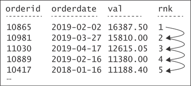
FIGURE 1-3 Basic understanding of the calculation of rank values.
Again, although this type of thinking leads to the correct result, it’s not entirely correct. In fact, making my point is even more difficult because the process I just described is actually very similar to how SQL Server physically handles the rank calculation. However, my focus at this point is not the physical implementation but rather the conceptual layer—the language and the logical model. When I discuss the “incorrect type of thinking,” I mean conceptually, from a language perspective, the calculation is thought of differently, in a set-based manner—not iterative. Remember that the language is not concerned with the physical implementation in the database engine. The physical layer’s responsibility is to figure out how to handle the logical request and both produce a correct result and produce it as fast as possible.
So, let me attempt to explain what I mean by the deeper, more correct understanding of how the language thinks of window functions. The function logically defines—for each row in the result set of the query—a separate, independent window. Absent any restrictions in the window specification, each window consists of the set of all rows from the result set of the query as the starting point. However, you can add elements to the window specification (for example, partitioning, framing, and so on) that will further restrict the set of rows in each window. (I’ll discuss partitioning and framing in more detail later.) Figure 1-4 shows a graphical depiction of this idea as it applies to our query with the RANK function.
)
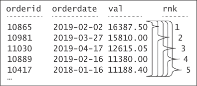
FIGURE 1-4 Deep understanding of the calculation of rank values.
With respect to each window function and row in the result set of the query, the OVER clause conceptually creates a separate window. In our query, we have not restricted the window specification in any way; we just defined the ordering specification for the calculation. So, in our case, all windows are made of all rows in the result set. They all coexist at the same time. In each, the rank is calculated as one more than the number of rows that have a greater value in the val attribute than the current value.
As you might realize, it’s more intuitive for many to think in the basic terms of the data being in an order and a process iterating through the rows one at a time. That’s okay when you’re starting out with window functions because you get to write your queries—or at least the simple ones—correctly. As time goes by, you can gradually transition to the deeper understanding of the window functions’ conceptual design and start thinking in a set-based manner.
Drawbacks of Alternatives to Window Functions
Window functions have several advantages compared to more traditional set-based alternative ways to achieve the same calculations—for example, grouped queries, subqueries, and others. Here, I’ll provide a couple of straightforward examples. There are several other important differences beyond the advantages I’ll show here, but it’s premature to discuss those now.
I’ll start with traditional grouped queries. Those do give you insight into new information in the form of aggregates, but you also lose something—the detail.
Once you group data, you’re forced to apply all calculations in the context of the group. But what if you need to apply calculations that involve both detail and aggregates? For example, suppose that you need to query the Sales.OrderValues view and calculate for each order the percentage of the current order value of the customer total, as well as the difference from the customer average. The current order value is a detail element, and the customer total and average are aggregates. If you group the data by customer, you don’t have access to the individual order values. One way to handle this need with traditional grouped queries is to have a query that groups the data by customer, define a table expression based on this query, and then join the table expression with the base table to match the detail with the aggregates. Listing 1-1 shows a query that implements this approach.
Listing 1-1 Mixing Detail and the Result of a Grouped Query
WITH Aggregates AS
(
  SELECT custid, SUM(val) AS sumval, AVG(val) AS avgval
  FROM Sales.OrderValues
  GROUP BY custid
)
SELECT O.orderid, O.custid, O.val,
  CAST(100. * O.val / A.sumval AS NUMERIC(5, 2)) AS pctcust,
  O.val - A.avgval AS diffcust
FROM Sales.OrderValues AS O
  INNER JOIN Aggregates AS A
    ON O.custid = A.custid;
Here’s the abbreviated output generated by the query shown in Listing 1-1:
orderid  custid  val     pctcust  diffcust
-------- ------- ------- -------- ------------
10835    1       845.80  19.79    133.633334
10952    1       471.20  11.03    -240.966666
10643    1       814.50  19.06    102.333334
10692    1       878.00  20.55    165.833334
11011    1       933.50  21.85    221.333334
10702    1       330.00  7.72     -382.166666
10625    2       479.75  34.20    129.012500
10759    2       320.00  22.81    -30.737500
10308    2       88.80   6.33     -261.937500
10926    2       514.40  36.67    163.662500
...
Now imagine needing to also involve the percentage from the grand total and the difference from the grand average. To do this, you need to add another table expression, as shown in Listing 1-2.
Listing 1-2 Mixing Detail and the Results of Two Grouped Queries
WITH CustAggregates AS
(
  SELECT custid, SUM(val) AS sumval, AVG(val) AS avgval
  FROM Sales.OrderValues
  GROUP BY custid
),
GrandAggregates AS
(
  SELECT SUM(val) AS sumval, AVG(val) AS avgval
  FROM Sales.OrderValues
)
SELECT O.orderid, O.custid, O.val,
  CAST(100. * O.val / CA.sumval AS NUMERIC(5, 2)) AS pctcust,
  O.val - CA.avgval AS diffcust,
  CAST(100. * O.val / GA.sumval AS NUMERIC(5, 2)) AS pctall,
  O.val - GA.avgval AS diffall
FROM Sales.OrderValues AS O
  INNER JOIN CustAggregates AS CA
    ON O.custid = CA.custid
  CROSS JOIN GrandAggregates AS GA;
Here’s the output of the query shown in Listing 1-2:
orderid  custid  val     pctcust  diffcust     pctall  diffall
-------- ------- ------- -------- ------------ ------- -------------
10835    1       845.80  19.79    133.633334   0.07    -679.252072
10952    1       471.20  11.03    -240.966666  0.04    -1053.852072
10643    1       814.50  19.06    102.333334   0.06    -710.552072
10692    1       878.00  20.55    165.833334   0.07    -647.052072
11011    1       933.50  21.85    221.333334   0.07    -591.552072
10702    1       330.00  7.72     -382.166666  0.03    -1195.052072
10625    2       479.75  34.20    129.012500   0.04    -1045.302072
10759    2       320.00  22.81    -30.737500   0.03    -1205.052072
10308    2       88.80   6.33     -261.937500  0.01    -1436.252072
10926    2       514.40  36.67    163.662500   0.04    -1010.652072
...
You can see how the query gets more and more complicated, involving more table expressions and more joins.
Another way to perform similar calculations is to use a separate subquery for each calculation. Listing 1-3 shows the alternatives, using subqueries to the last two grouped queries.
Listing 1-3 Mixing Detail and the Results of Scalar Aggregate Subqueries
-- subqueries, detail and cust aggregates
SELECT orderid, custid, val,
  CAST(100. * val /
        (SELECT SUM(O2.val)
         FROM Sales.OrderValues AS O2
         WHERE O2.custid = O1.custid) AS NUMERIC(5, 2)) AS pctcust,
  val - (SELECT AVG(O2.val)
         FROM Sales.OrderValues AS O2
         WHERE O2.custid = O1.custid) AS diffcust
FROM Sales.OrderValues AS O1;

-- subqueries, detail, customer and grand aggregates
SELECT orderid, custid, val,
  CAST(100. * val /
        (SELECT SUM(O2.val)
         FROM Sales.OrderValues AS O2
         WHERE O2.custid = O1.custid) AS NUMERIC(5, 2)) AS pctcust,
  val - (SELECT AVG(O2.val)
         FROM Sales.OrderValues AS O2
         WHERE O2.custid = O1.custid) AS diffcust,
  CAST(100. * val /
        (SELECT SUM(O2.val)
         FROM Sales.OrderValues AS O2) AS NUMERIC(5, 2)) AS pctall,
  val - (SELECT AVG(O2.val)
         FROM Sales.OrderValues AS O2) AS diffall
FROM Sales.OrderValues AS O1;
There are two main problems with the subquery approach. First, you end up with lengthy complex code. Second, SQL Server’s optimizer is not coded at the moment to identify cases where multiple subqueries need to access the same set of rows; hence, it will use separate visits to the data for each subquery. This means that the more subqueries you have, the more visits to the data you get. Unlike the previous problem, this one is not a problem with the language, but rather with the specific optimization you get for subqueries in SQL Server.
Remember that the idea behind a window function is to define a window, or a set, of rows for the function to operate on. Aggregate functions are supposed to be applied to a set of rows; therefore, the concept of windowing can work well with those as an alternative to using grouping or subqueries. And when calculating the aggregate window function, you don’t lose the detail. You use the OVER clause to define the window for the function. For example, to calculate the sum of all values from the result set of the query, simply use the following expression:
SUM(val) OVER()
If you do not restrict the window (empty parentheses), your starting point is the result set of the query.
To calculate the sum of all values from the result set of the query where the customer ID is the same as in the current row, use the partitioning capabilities of window functions (which I’ll say more about later) and partition the window by custid, as follows:
SUM(val) OVER(PARTITION BY custid)
Note that within window functions, the term partitioning suggests a filter because it limits the rows that the function operates on compared to the complete, nonpartitioned, window.
Using window functions, here’s how you address the request involving the detail and customer aggregates, returning the percentage of the current order value of the customer total as well as the difference from the average (with window functions in bold):
SELECT orderid, custid, val,
   CAST(100. * val / SUM(val) OVER(PARTITION BY custid) AS NUMERIC(5, 2)) AS pctcust,
   val - AVG(val) OVER(PARTITION BY custid) AS diffcust
FROM Sales.OrderValues;
And here’s another query where you also add the percentage of the grand total and the difference from the grand average:
SELECT orderid, custid, val,
   CAST(100. * val / SUM(val) OVER(PARTITION BY custid) AS NUMERIC(5, 2)) AS pctcust,
   val - AVG(val) OVER(PARTITION BY custid) AS diffcust,
   CAST(100. * val / SUM(val) OVER() AS NUMERIC(5, 2)) AS pctall,
   val - AVG(val) OVER() AS diffall
FROM Sales.OrderValues;
Observe how much simpler and more concise the versions with the window functions are. Also, in terms of optimization, note that SQL Server’s optimizer was coded with the logic to look for multiple functions with the same window specification. If any are found, SQL Server will use the same visit to the data for those. For example, in the last query, SQL Server will use one visit to the data to calculate the first two functions (the sum and average that are partitioned by custid), and it will use one other visit to calculate the last two functions (the sum and average that are nonpartitioned). I will demonstrate this concept of optimization in Chapter 5, “Optimization of Window Functions.”
Another advantage window functions have over subqueries is that the initial window prior to applying restrictions is the result set of the query. This means that it’s the result set after applying table operators (for example, joins), row filters (the WHERE clause), grouping, and group filtering (the HAVING clause). You get this result set because of the phase of logical query processing in which window functions get evaluated. (I’ll say more about this later in this chapter.) Conversely, a subquery starts from scratch—not from the result set of the underlying query. This means that if you want the subquery to operate on the same set as the result of the underlying query, it will need to repeat all query constructs used by the underlying query. As an example, suppose that you want our calculations of the percentage of the total and the difference from the average to apply only to orders placed in the year 2018. With the solution using window functions, all you need to do is add one filter to the query, like so:
SELECT orderid, custid, val,
  CAST(100. * val / SUM(val) OVER(PARTITION BY custid) AS NUMERIC(5, 2)) AS pctcust,
  val - AVG(val) OVER(PARTITION BY custid) AS diffcust,
  CAST(100. * val / SUM(val) OVER() AS NUMERIC(5, 2)) AS pctall,
  val - AVG(val) OVER() AS diffall
FROM Sales.OrderValues
WHERE orderdate >= '20180101'
  AND orderdate < '20190101';
The starting point for all window functions is the set after applying the filter. But with subqueries, you start from scratch; therefore, you need to repeat the filter in all of your subqueries, as shown in Listing 1-4.
Listing 1-4 Repeating Filter in All Subqueries
SELECT orderid, custid, val,
  CAST(100. * val /
        (SELECT SUM(O2.val)
         FROM Sales.OrderValues AS O2
         WHERE O2.custid = O1.custid
           AND orderdate >= '20180101'
           AND orderdate < '20190101') AS NUMERIC(5, 2)) AS pctcust,
  val - (SELECT AVG(O2.val)
         FROM Sales.OrderValues AS O2
         WHERE O2.custid = O1.custid
           AND orderdate >= '20180101'
           AND orderdate < '20190101') AS diffcust,
  CAST(100. * val /
        (SELECT SUM(O2.val)
         FROM Sales.OrderValues AS O2
         WHERE orderdate >= '20180101'
           AND orderdate < '20190101') AS NUMERIC(5, 2)) AS pctall,
  val - (SELECT AVG(O2.val)
         FROM Sales.OrderValues AS O2
         WHERE orderdate >= '20180101'
           AND orderdate < '20190101') AS diffall
FROM Sales.OrderValues AS O1
WHERE orderdate >= '20180101'
  AND orderdate < '20190101';
Of course, you could use workarounds, such as first defining a common table expression (CTE) based on a query that performs the filter, and then have both the outer query and the subqueries refer to the CTE. However, my point is that with window functions, you don’t need any workarounds because they operate on the result of the query. I will provide more details about this aspect in the design of window functions later in the chapter (see “Window Functions”).
As mentioned earlier, window functions also lend themselves to good optimization, and often, alternatives to window functions don’t get optimized as well, to say the least. Of course, there are cases where the inverse is also true. I explain the optimization of window functions in Chapter 5 and provide plenty of examples for using them efficiently in Chapter 6.