Manage workbook options and settings
- By Paul McFedries
- 2/1/2017
- Objective 1.2: Manage workbook review
- Objective 1.2 practice tasks
In this sample chapter from MOS 2016 Study Guide for Microsoft Excel Expert, learn how to use worksheet protection features to prevent changes to a single cell or entire workbook in Microsoft Excel 2016.
Objective 1.2: Manage workbook review
Restrict editing
When you have labored long and hard to get your worksheet formulas or formatting just right, the last thing you need is to have a cell or range accidentally deleted or copied over. You can prevent this problem by using Excel’s worksheet protection features, which you can use to prevent changes to anything from a single cell to an entire workbook.
For protecting cells, Excel offers two techniques:
Protection formatting When you use this technique, you format those cells in which you want to allow editing as unlocked, and you format all other cells as locked. You can also hide the formulas in one or more cells if you don’t want users to see them. You then turn on worksheet protection, which means that locked cells can’t be changed, deleted, moved, or copied over, and that hidden formulas are no longer visible.
Protect a range with a password When you use this technique, you protect one or more ranges with a password, and then specify which users are allowed or denied editing privileges on that range.
By default, all worksheet cells are formatted as locked and their formulas are visible. Note, however, that “locked” in this context really only means that the cells have the potential to be locked. That’s because Excel doesn’t perform the actual lock—that is, it doesn’t prevent users from modifying the cells—until you turn on worksheet protection. With this in mind, here are the options you have when setting up your protection formatting:
If you want to protect every cell, you can leave the formatting as it is and turn on worksheet protection.
If you want only certain cells to be unlocked (for data entry, for example), you can select those cells and unlock them before turning on worksheet protection. Similarly, if you want certain formulas hidden, you can select the cells and hide their formulas.
If you want only certain cells to be locked, first select all the cells and unlock them. Then select the cells you want protected and lock them. To keep only selected formulas visible, hide every formula and then make the formulas you want visible.
If you don’t want to protect the entire worksheet, you can restrict your protection to a more targeted area. That is, if you want to prevent unauthorized users from editing within a specific range, you can set up that range with a password. After you protect the sheet, only authorized users who know the password can edit the range.
When you set up protection formatting on one or more cells, or protect one or more ranges with a password, your restrictions don’t go into effect until you activate worksheet protection.
To unlock worksheet cells
Select the cells you want to unlock.
On the Home tab, in the Cells group, click Format, and then click to deactivate the Lock Cell command.
To lock only certain worksheet cells
Select all the cells in the worksheet.
On the Home tab, click Format, and then click to deactivate the Lock Cell command.
Select the cells you want to lock.
On the Home tab, click Format, and then click to activate the Lock Cell command.
To hide formulas in worksheet cells
Select the cells that contain the formulas you want to hide.
On the Home tab, click Format, and then click Format Cells.
In the Format Cells dialog box, on the Protection tab, select the Hidden check box, and then click OK.
To show only certain formulas in worksheet cells
Select all the cells in the worksheet.
On the Home tab, click Format, and then click Format Cells.
In the Format Cells dialog box, on the Protection tab, select the Hidden check box, and then click OK.
On the worksheet, select the cells that contain the formulas you want to show.
On the Home tab, click Format, and then click Format Cells.
In the Format Cells dialog box, on the Protection tab, clear the Hidden check box, and then click OK.
To protect a range with a password
On the Review tab, in the Changes group, click Allow Users to Edit Ranges.
In the Allow Users to Edit Ranges dialog box, click New to open the New Range dialog box.
In the Title box, enter a name for the range.
In the Refers to cells box, enter or select the range you want to protect.
In the Range password box, enter a password.
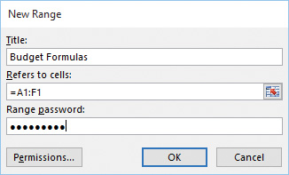
Name, specify, and password-protect a range in the New Range dialog box
If you want the password requirement to apply to only specific users or groups, click Permissions, and then in the Permissions dialog box, do the following:
Click Add, enter the name of a user or group, and then click OK to add the user or group to the Permissions dialog box.
Click the user or group, and then for the Edit range without a password permission, select the Deny check box.
Click OK to return to the New Range dialog box.
In the New Range dialog box, click OK, reenter the password to confirm it, and then click OK. Excel adds the range to the Allow Users To Edit Ranges dialog box.
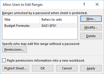
Your protected ranges appear in the Allow Users To Edit Ranges dialog box
Repeat steps 2 through 7 to protect other ranges, and then click OK to close the dialog box and save your changes.
To activate worksheet protection
Do either of the following to open the Protect Sheet dialog box:
On the Review tab, in the Changes group, click Protect Sheet.
If the Allow Users To Edit Ranges dialog box is open, click the Protect Sheet button in that dialog box.
In the Protect Sheet dialog box, do the following, and then click OK:
Select the Protect worksheet and contents of locked cells check box.
If you want, for added security, enter a password in the Password to unprotect sheet box. This means that no one can turn off the worksheet’s protection without first entering the password.
In the Allow all users of this worksheet to list, select the check box beside each action you want unauthorized users to be allowed to perform.

Activate your protection formatting or range passwords in the Protect Sheet dialog box
If you entered a password, reenter the password, and then click OK to continue working in the worksheet.
Protect workbook structure
When you protect a workbook’s structure, Excel takes the following actions:
Disables most of the worksheet-related commands on the ribbon. For example, on the Home tab, on the Format menu, the Rename Sheet and Move Or Copy Sheet commands are unavailable.
Disables most of the commands on the worksheet tab’s shortcut menu, including Insert, Delete, Rename, and Move or Copy.
Keeps the Scenario Manager from creating a summary report.
To protect the workbook structure
In the workbook you want to protect, on the Review tab, in the Changes group, click Protect Workbook to display the Protect Structure And Windows dialog box.
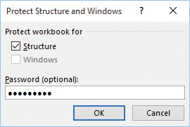
Use the Protect Structure And Windows dialog box to prevent changes to your workbook’s formatting and worksheet structure
Select the Structure check box.
Enter an optional password in the Password text box, and then click OK.
If you specified a password, reenter the password to confirm, and then click OK.
Encrypt a workbook with a password
For a workbook with confidential data, merely protecting cells or sheets might not be enough. For a higher level of security, you can encrypt the workbook with a password. This prevents anyone who doesn’t know the password from opening the workbook.
To encrypt a workbook with a password
In the workbook you want to protect, display the Info page of the Backstage view.
Click Protect Workbook, and then click Encrypt with Password.
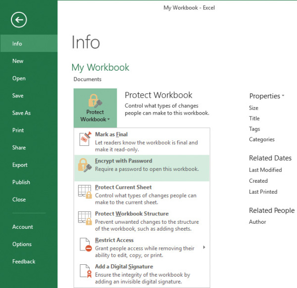
Use the Encrypt With Password command to protect your workbook with a password
Enter a password, and then click OK.
Confirm the password, and then click OK.
)
Manage workbook versions
On occasion, you might realize that you have improperly edited some workbook data, or you have accidentally overwritten an important worksheet range during a paste operation. In some circumstances, you can use the following methods to recover:
If the improper edit or paste was the most recent action you performed, you can use Undo to reverse the action.
If the error was not the most recent action, but you don’t need to preserve any workbook changes you’ve made since then, you can repeatedly use Undo until the mistaken action is reversed.
If you haven’t saved the workbook since you made the error, and you don’t need to preserve any changes you’ve made since the last save operation, you can close the workbook without saving it.
Unfortunately, these three scenarios don’t always apply when you want to revert a workbook to an earlier state. For example, closing the workbook without saving changes might cause you to lose too much work if you haven’t saved the file in a while. However, if you have Excel’s AutoRecover feature running, Excel is monitoring your workbook for changes. Each time the AutoRecover interval ends (which is, by default, every 10 minutes), if Excel sees that your workbook has unsaved changes, it saves a copy of the workbook. This means that you can often reverse an error without losing too much work by reverting to an earlier autosaved version of the workbook.
To configure AutoRecover
In the Excel Options dialog box, on the Save page, select the Save AutoRecover information every X minutes check box.
Use the arrows to set the AutoRecover interval, in minutes.
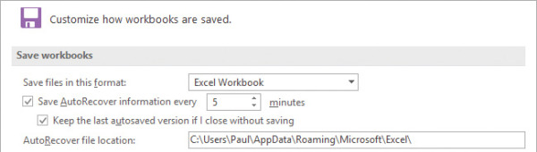
Use the Save page of the Excel Options dialog box to configure the AutoRecover settings
To have Excel preserve the most recent autosaved version of any workbook that you close with unsaved changes, select the Keep the last autosaved version if I close without saving check box.
In the AutoRecover file location box, you can optionally enter the path of a different folder in which Excel should store the autosaved versions.
Click OK.
)
To revert to an earlier version of a workbook
On the Info page of the Backstage view, under Manage Workbook, click the autosaved version of the workbook to which you want to revert.
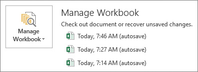
On the Info page, click one of the autosaved versions that appear under the Manage Workbook heading
If this is the version you want to recover, display the Save As page to save the workbook under a different file name or in a different folder; otherwise, you can return to the most recent version by clicking Restore in the information bar.
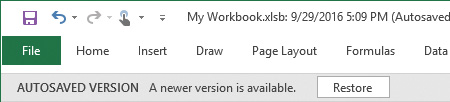
You can return from an autosaved version of a workbook to the most recent version by clicking Restore
Configure formula calculation options
Excel always calculates a formula when you confirm its entry, and the program normally recalculates existing formulas automatically whenever their data changes. This behavior is fine for small worksheets, but it can slow you down if you have a complex model that takes several seconds or even several minutes to recalculate. To turn off this automatic recalculation, Excel gives you two ways to get started:
You can use commands on the Calculation Options menu on the Formula tab.
You can use settings on the Formulas page of the Excel Options dialog box.
Either way, you’re presented with three calculation options:
Automatic This is the default calculation mode; it means that Excel recalculates formulas as soon as you enter them and as soon as the data for a formula changes.
Automatic except for data tables In this calculation mode, Excel recalculates all formulas automatically, except for those associated with data tables. This is a good choice if your worksheet includes one or more massive data tables that are slowing down the recalculation.
Manual Select this mode to force Excel not to recalculate any formulas until you either manually recalculate or save the workbook.
With manual calculation turned on, Calculate appears in the status bar whenever your worksheet data changes and your formula results need to be updated.
You can also control various options for iterative calculations. These are calculations where you begin with a guess at the solution, plug that guess into the formula to get a new solution, plug that solution into the formula, and then keep repeating this procedure. Each time you plug a new solution into the formula it is called an iteration, so the entire process is called an iterative calculation. This type of calculation creates a circular reference, which is normally an error in Excel, so that’s why iterative calculations are turned off by default.
How does an iterative calculation know when to stop? If during the iterative process the change from one solution to the next becomes smaller than some predetermined value, the formula is said to have converged on the solution. Because the formula might not ever converge—or it might only converge after an unacceptably large number of iterations—you can also tell Excel to stop after a predetermined number of iterations.
To enable the management of iterative calculations, the Formulas tab in the Excel Options dialog box offers two controls:
Maximum Iterations This value is the number of iterations after which Excel must stop the calculation if it hasn’t yet converged to a solution. The default value is 100.
Maximum Change This value is the threshold that Excel uses to determine whether the iterative calculation has converged on a solution. If the change in the formula result from one iteration is less than this value, Excel considers the formula solved and stops the iteration. The default value is 0.001, but you can reduce this (for example, to 0.0001 or 0.00001) if you require a solution with more precision.
When performing an iterative calculation, Excel stops the calculation as soon as it hits the Maximum Iterations value or the Maximum Change value (whichever comes first).
To configure the formula calculation options
On the Formulas tab, in the Calculation group, click Calculation Options, and then click Automatic, Automatic Except for Data Tables, or Manual.
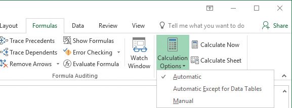
Choose how you want Excel to calculate workbook formulas
Or
In the Excel Options dialog box, on the Formulas page, under Workbook Calculation, select the option you want.
If you select the Manual option and want to run the calculation automatically when you save the file, select the Recalculate workbook before saving check box.
Click OK.
)
To manually recalculate a single formula
Select the cell containing the formula.
Click in the formula bar, and then press Enter or click the Enter button.
To manually recalculate formulas in a selected cell range
Display the Replace tab of the Find and Replace dialog box:
Enter an equal sign (=) in both the Find What and Replace With boxes.
Click Replace All.
To manually recalculate formulas in only the active worksheet
On the Formulas tab, click Calculate Sheet.
Press Shift+F9.
To manually recalculate formulas in every open worksheet
On the Formulas tab, in the Calculation group, click Calculate Now.
Press F9.
To manually recalculate every formula in every open worksheet
Press Ctrl+Alt+Shift+F9.
To enable and configure iterative calculations
In the Excel Options dialog box, on the Formulas page, select the Enable iterative calculation check box.
In the Maximum Iterations box, enter or select the number of iterations Excel can try before it must stop the calculation.
In the Maximum Change box, enter the numeric value that you want Excel to use as a threshold to determine whether the calculation has converged on a solution.
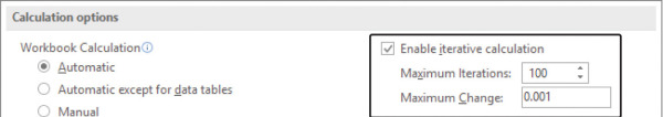
Enable and configure iterative calculations on the Formulas page of the Excel Options dialog box
Click OK.
)