Background to T-SQL querying and programming
- By Itzik Ben-Gan
- 10/7/2016
- Theoretical background
- SQL Server architecture
- Creating tables and defining data integrity
- Conclusion
Learning the theory behind T-SQL querying and programming is an important step in developing code. In this sample chapter from T-SQL Fundamentals, 3rd Edition, Itzik Ben-Gan provides a brief theoretical background about SQL, set theory and predicate logic, the relational model, and types of database systems.
You’re about to embark on a journey to a land that is like no other—a land that has its own set of laws. If reading this book is your first step in learning Transact-SQL (T-SQL), you should feel like Alice—just before she started her adventures in Wonderland. For me, the journey has not ended; instead, it’s an ongoing path filled with new discoveries. I envy you; some of the most exciting discoveries are still ahead of you!
I’ve been involved with T-SQL for many years: teaching, speaking, writing, and consulting about it. For me, T-SQL is more than just a language—it’s a way of thinking. In my first few books about T-SQL, I’ve written extensively on advanced topics, and for years, I have postponed writing about fundamentals. This is not because T-SQL fundamentals are simple or easy—in fact, it’s just the opposite. The apparent simplicity of the language is misleading. I could explain the language syntax elements in a superficial manner and have you writing queries within minutes. But that approach would only hold you back in the long run and make it harder for you to understand the essence of the language.
Acting as your guide while you take your first steps in this realm is a big responsibility. I wanted to make sure that I spent enough time and effort exploring and understanding the language before writing about fundamentals. T-SQL is deep; learning the fundamentals the right way involves much more than just understanding the syntax elements and coding a query that returns the right output. You pretty much need to forget what you know about other programming languages and start thinking in terms of T-SQL.
Theoretical background
SQL stands for Structured Query Language. SQL is a standard language that was designed to query and manage data in relational database management systems (RDBMSs). An RDBMS is a database management system based on the relational model (a semantic model for representing data), which in turn is based on two mathematical branches: set theory and predicate logic. Many other programming languages and various aspects of computing evolved pretty much as a result of intuition. In contrast, to the degree that SQL is based on the relational model, it is based on a firm foundation—applied mathematics. T-SQL thus sits on wide and solid shoulders. Microsoft provides T-SQL as a dialect of, or extension to, SQL in Microsoft SQL Server data-management software, its RDBMS.
This section provides a brief theoretical background about SQL, set theory and predicate logic, the relational model, and types of database systems. Because this book is neither a mathematics book nor a design/data-modeling book, the theoretical information provided here is informal and by no means complete. The goals are to give you a context for the T-SQL language and to deliver the key points that are integral to correctly understanding T-SQL later in the book.
SQL
SQL is both an ANSI and ISO standard language based on the relational model, designed for querying and managing data in an RDBMS.
In the early 1970s, IBM developed a language called SEQUEL (short for Structured English QUEry Language) for its RDBMS product called System R. The name of the language was later changed from SEQUEL to SQL because of a trademark dispute. SQL first became an ANSI standard in 1986, and then an ISO standard in 1987. Since 1986, the American National Standards Institute (ANSI) and the International Organization for Standardization (ISO) have been releasing revisions for the SQL standard every few years. So far, the following standards have been released: SQL-86 (1986), SQL-89 (1989), SQL-92 (1992), SQL:1999 (1999), SQL:2003 (2003), SQL:2006 (2006), SQL:2008 (2008), and SQL:2011 (2011). The SQL standard is made of multiple parts. Part 1 (Framework) and Part 2 (Foundation) pertain to the SQL language, whereas the other parts define standard extensions, such as SQL for XML and SQL-Java integration.
Interestingly, SQL resembles English and is also very logical. Unlike many programming languages, which use an imperative programming paradigm, SQL uses a declarative one. That is, SQL requires you to specify what you want to get and not how to get it, letting the RDBMS figure out the physical mechanics required to process your request.
SQL has several categories of statements, including Data Definition Language (DDL), Data Manipulation Language (DML), and Data Control Language (DCL). DDL deals with object definitions and includes statements such as CREATE, ALTER, and DROP. DML allows you to query and modify data and includes statements such as SELECT, INSERT, UPDATE, DELETE, TRUNCATE, and MERGE. It’s a common misunderstanding that DML includes only data-modification statements, but as I mentioned, it also includes SELECT. Another common misunderstanding is that TRUNCATE is a DDL statement, but in fact it is a DML statement. DCL deals with permissions and includes statements such as GRANT and REVOKE. This book focuses on DML.
T-SQL is based on standard SQL, but it also provides some nonstandard/proprietary extensions. Moreover, T-SQL does not implement all of standard SQL. In other words, T-SQL is both a subset and a superset of SQL. When describing a language element for the first time, I’ll typically mention whether it is standard.
Set theory
Set theory, which originated with the mathematician Georg Cantor, is one of the mathematical branches on which the relational model is based. Cantor’s definition of a set follows:
By a “set” we mean any collection M into a whole of definite, distinct objects m (which are called the “elements” of M) of our perception or of our thought.
—Joseph W. Dauben and Georg Cantor (Princeton University Press, 1990)
Every word in the definition has a deep and crucial meaning. The definitions of a set and set membership are axioms that are not supported by proofs. Each element belongs to a universe, and either is or is not a member of the set.
Let’s start with the word whole in Cantor’s definition. A set should be considered a single entity. Your focus should be on the collection of objects as opposed to the individual objects that make up the collection. Later on, when you write T-SQL queries against tables in a database (such as a table of employees), you should think of the set of employees as a whole rather than the individual employees. This might sound trivial and simple enough, but apparently many programmers have difficulty adopting this way of thinking.
The word distinct means that every element of a set must be unique. Jumping ahead to tables in a database, you can enforce the uniqueness of rows in a table by defining key constraints. Without a key, you won’t be able to uniquely identify rows, and therefore the table won’t qualify as a set. Rather, the table would be a multiset or a bag.
The phrase of our perception or of our thought implies that the definition of a set is subjective. Consider a classroom: one person might perceive a set of people, whereas another might perceive a set of students and a set of teachers. Therefore, you have a substantial amount of freedom in defining sets. When you design a data model for your database, the design process should carefully consider the subjective needs of the application to determine adequate definitions for the entities involved.
As for the word object, the definition of a set is not restricted to physical objects, such as cars or employees, but rather is relevant to abstract objects as well, such as prime numbers or lines.
What Cantor’s definition of a set leaves out is probably as important as what it includes. Notice that the definition doesn’t mention any order among the set elements. The order in which set elements are listed is not important. The formal notation for listing set elements uses curly brackets: {a, b, c}. Because order has no relevance, you can express the same set as {b, a, c} or {b, c, a}. Jumping ahead to the set of attributes (called columns in SQL) that make up the heading of a relation (called a table in SQL), an element is supposed to be identified by name—not by ordinal position.
Similarly, consider the set of tuples (called rows by SQL) that make up the body of the relation; an element is identified by its key values—not by position. Many programmers have a hard time adapting to the idea that, with respect to querying tables, there is no order among the rows. In other words, a query against a table can return table rows in any order unless you explicitly request that the data be sorted in a specific way, perhaps for presentation purposes.
Predicate logic
Predicate logic, whose roots reach back to ancient Greece, is another branch of mathematics on which the relational model is based. Dr. Edgar F. Codd, in creating the relational model, had the insight to connect predicate logic to both the management and querying of data. Loosely speaking, a predicate is a property or an expression that either holds or doesn’t hold—in other words, is either true or false. The relational model relies on predicates to maintain the logical integrity of the data and define its structure. One example of a predicate used to enforce integrity is a constraint defined in a table called Employees that allows only employees with a salary greater than zero to be stored in the table. The predicate is “salary greater than zero” (T-SQL expression: salary > 0).
You can also use predicates when filtering data to define subsets, and more. For example, if you need to query the Employees table and return only rows for employees from the sales department, you use the predicate “department equals sales” in your query filter (T-SQL expression: department = ‘sales’).
In set theory, you can use predicates to define sets. This is helpful because you can’t always define a set by listing all its elements (for example, infinite sets), and sometimes for brevity it’s more convenient to define a set based on a property. As an example of an infinite set defined with a predicate, the set of all prime numbers can be defined with the following predicate: “x is a positive integer greater than 1 that is divisible only by 1 and itself.” For any specified value, the predicate is either true or not true. The set of all prime numbers is the set of all elements for which the predicate is true. As an example of a finite set defined with a predicate, the set {0, 1, 2, 3, 4, 5, 6, 7, 8, 9} can be defined as the set of all elements for which the following predicate holds true: “x is an integer greater than or equal to 0 and smaller than or equal to 9.”
The relational model
The relational model is a semantic model for data management and manipulation and is based on set theory and predicate logic. As mentioned earlier, it was created by Dr. Edgar F. Codd, and later explained and developed by Chris Date, Hugh Darwen, and others. The first version of the relational model was proposed by Codd in 1969 in an IBM research report called “Derivability, Redundancy, and Consistency of Relations Stored in Large Data Banks.” A revised version was proposed by Codd in 1970 in a paper called “A Relational Model of Data for Large Shared Data Banks,” published in the journal Communications of the ACM.
The goal of the relational model is to enable consistent representation of data with minimal or no redundancy and without sacrificing completeness, and to define data integrity (enforcement of data consistency) as part of the model. An RDBMS is supposed to implement the relational model and provide the means to store, manage, enforce the integrity of, and query data. The fact that the relational model is based on a strong mathematical foundation means that given a certain data-model instance (from which a physical database will later be generated), you can tell with certainty when a design is flawed, rather than relying solely on intuition.
The relational model involves concepts such as propositions, predicates, relations, tuples, attributes, and more. For nonmathematicians, these concepts can be quite intimidating. The sections that follow cover some key aspects of the model in an informal, nonmathematical manner and explain how they relate to databases.
Propositions, predicates, and relations
The common belief that the term relational stems from relationships between tables is incorrect. “Relational” actually pertains to the mathematical term relation. In set theory, a relation is a representation of a set. In the relational model, a relation is a set of related information, with the counterpart in SQL being a table—albeit not an exact counterpart. A key point in the relational model is that a single relation should represent a single set (for example, Customers). Note that operations on relations (based on relational algebra) result in a relation (for example, a join between two relations).
 NOTE
NOTE
The relational model distinguishes between a relation and a relation variable, but to keep things simple, I won’t get into this distinction. Instead, I’ll use the term relation for both cases. Also, a relation is made of a heading and a body. The heading consists of a set of attributes (called columns in SQL), where each element is identified by an attribute name and a type name. The body consists of a set of tuples (called rows in SQL), where each element is identified by a key. To keep things simple, I’ll refer to a table as a set of rows.
When you design a data model for a database, you represent all data with relations (tables). You start by identifying propositions that you will need to represent in your database. A proposition is an assertion or a statement that must be true or false. For example, the statement, “Employee Itzik Ben-Gan was born on February 12, 1971, and works in the IT department” is a proposition. If this proposition is true, it will manifest itself as a row in a table of Employees. A false proposition simply won’t manifest itself. This presumption is known as the closed-world assumption (CWA).
The next step is to formalize the propositions. You do this by taking out the actual data (the body of the relation) and defining the structure (the heading of the relation)—for example, by creating predicates out of propositions. You can think of predicates as parameterized propositions. The heading of a relation comprises a set of attributes. Note the use of the term “set”; in the relational model, attributes are unordered and distinct. An attribute is identified by an attribute name and a type name. For example, the heading of an Employees relation might consist of the following attributes (expressed as pairs of attribute names and type names): employeeid integer, firstname character string, lastname character string, birthdate date, and departmentid integer.
A type is one of the most fundamental building blocks for relations. A type constrains an attribute to a certain set of possible or valid values. For example, the type INT is the set of all integers in the range –2,147,483,648 to 2,147,483,647. A type is one of the simplest forms of a predicate in a database because it restricts the attribute values that are allowed. For example, the database would not accept a proposition where an employee birth date is February 31, 1971 (not to mention a birth date stated as something like “abc!”). Note that types are not restricted to base types such as integers or character strings; a type also can be an enumeration of possible values, such as an enumeration of possible job positions. A type can be simple or complex. Probably the best way to think of a type is as a class—encapsulated data and the behavior supporting it. An example of a complex type is a geometry type that supports polygons.
Missing values
One aspect of the relational model is the source of many passionate debates—whether predicates should be restricted to two-valued logic. That is, in two-valued predicate logic, a predicate is either true or false. If a predicate is not true, it must be false. Use of two-valued predicate logic follows a mathematical law called “the law of excluded middle.” However, some say that there’s room for three-valued (or even four-valued) predicate logic, taking into account cases where values are missing. A predicate involving a missing value yields neither true nor false—it yields unknown.
Take, for example, a mobile phone attribute of an Employees relation. Suppose that a certain employee’s mobile phone number is missing. How do you represent this fact in the database? In a three-valued logic implementation, the mobile phone attribute should allow the use of a special marker for a missing value. Then a predicate comparing the mobile phone attribute with some specific number will yield unknown for the case with the missing value. Three-valued predicate logic refers to the three possible logical values that can result from a predicate—true, false, and unknown.
Some people believe that three-valued predicate logic is nonrelational, whereas others believe that it is relational. Codd actually advocated for four-valued predicate logic, saying that there were two different cases of missing values: missing but applicable (A-Values marker), and missing but inapplicable (I-Values marker). An example of “missing but applicable” is when an employee has a mobile phone, but you don’t know what the mobile phone number is. An example of “missing but inapplicable” is when an employee doesn’t have a mobile phone at all. According to Codd, two special markers should be used to support these two cases of missing values. SQL implements three-valued predicate logic by supporting the NULL marker to signify the generic concept of a missing value. Support for NULLs and three-valued predicate logic in SQL is the source of a great deal of confusion and complexity, though one can argue that missing values are part of reality. In addition, the alternative—using only two-valued predicate logic—is no less problematic.
NOTE
As mentioned, a NULL is not a value but rather a marker for a missing value. Therefore, though unfortunately it’s common, the use of the terminology “NULL value” is incorrect. The correct terminology is “NULL marker” or just “NULL.” In the book, I chose to use the latter because it’s more common in the SQL community.
Constraints
One of the greatest benefits of the relational model is the ability to define data integrity as part of the model. Data integrity is achieved through rules called constraints that are defined in the data model and enforced by the RDBMS. The simplest methods of enforcing integrity are assigning an attribute type with its attendant “nullability” (whether it supports or doesn’t support NULLs). Constraints are also enforced through the model itself; for example, the relation Orders(orderid, orderdate, duedate, shipdate) allows three distinct dates per order, whereas the relations Employees(empid) and EmployeeChildren(empid, childname) allow zero to countable infinity children per employee.
Other examples of constraints include candidate keys, which provide entity integrity, and foreign keys, which provide referential integrity. A candidate key is a key defined on one or more attributes that prevents more than one occurrence of the same tuple (row in SQL) in a relation. A predicate based on a candidate key can uniquely identify a row (such as an employee). You can define multiple candidate keys in a relation. For example, in an Employees relation, you can define candidate keys on employeeid, on SSN (Social Security number), and others. Typically, you arbitrarily choose one of the candidate keys as the primary key (for example, employeeid in the Employees relation) and use that as the preferred way to identify a row. All other candidate keys are known as alternate keys.
Foreign keys are used to enforce referential integrity. A foreign key is defined on one or more attributes of a relation (known as the referencing relation) and references a candidate key in another (or possibly the same) relation. This constraint restricts the values in the referencing relation’s foreign-key attributes to the values that appear in the referenced relation’s candidate-key attributes. For example, suppose that the Employees relation has a foreign key defined on the attribute departmentid, which references the primary-key attribute departmentid in the Departments relation. This means that the values in Employees.departmentid are restricted to the values that appear in Departments.departmentid.
Normalization
The relational model also defines normalization rules (also known as normal forms). Normalization is a formal mathematical process to guarantee that each entity will be represented by a single relation. In a normalized database, you avoid anomalies during data modification and keep redundancy to a minimum without sacrificing completeness. If you follow Entity Relationship Modeling (ERM), and represent each entity and its attributes, you probably won’t need normalization; instead, you will apply normalization only to reinforce and ensure that the model is correct. You can find the definition of ERM in the following Wikipedia article: https://en.wikipedia.org/wiki/Entity%E2%80%93relationship_model.
The following sections briefly cover the first three normal forms (1NF, 2NF, and 3NF) introduced by Codd.
1NF
The first normal form says that the tuples (rows) in the relation (table) must be unique and attributes should be atomic. This is a redundant definition of a relation; in other words, if a table truly represents a relation, it is already in first normal form.
You achieve unique rows in SQL by defining a unique key for the table.
You can operate on attributes only with operations that are defined as part of the attribute’s type. Atomicity of attributes is subjective in the same way that the definition of a set is subjective. As an example, should an employee name in an Employees relation be expressed with one attribute (fullname), two (firstname and lastname), or three (firstname, middlename, and lastname)? The answer depends on the application. If the application needs to manipulate the parts of the employee’s name separately (such as for search purposes), it makes sense to break them apart; otherwise, it doesn’t.
In the same way that an attribute might not be atomic enough based on the needs of the applications that use it, an attribute might also be subatomic. For example, if an address attribute is considered atomic for the applications that use it, not including the city as part of the address would violate the first normal form.
This normal form is often misunderstood. Some people think that an attempt to mimic arrays violates the first normal form. An example would be defining a YearlySales relation with the following attributes: salesperson, qty2014, qty2015, and qty2016. However, in this example, you don’t really violate the first normal form; you simply impose a constraint—restricting the data to three specific years: 2014, 2015, and 2016.
2NF
The second normal form involves two rules. One rule is that the data must meet the first normal form. The other rule addresses the relationship between nonkey and candidate-key attributes. For every candidate key, every nonkey attribute has to be fully functionally dependent on the entire candidate key. In other words, a nonkey attribute cannot be fully functionally dependent on part of a candidate key. To put it more informally, if you need to obtain any nonkey attribute value, you need to provide the values of all attributes of a candidate key from the same tuple. You can find any value of any attribute of any tuple if you know all the attribute values of a candidate key.
As an example of violating the second normal form, suppose that you define a relation called Orders that represents information about orders and order lines. (See Figure 1-1.) The Orders relation contains the following attributes: orderid, productid, orderdate, qty, customerid, and companyname. The primary key is defined on orderid and productid.
)
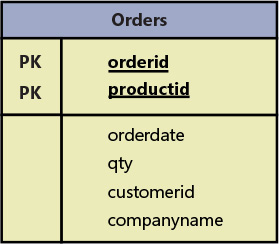
Figure 1-1 Data model before applying 2NF.
The second normal form is violated in Figure 1-1 because there are nonkey attributes that depend on only part of a candidate key (the primary key, in this example). For example, you can find the orderdate of an order, as well as customerid and companyname, based on the orderid alone.
To conform to the second normal form, you would need to split your original relation into two relations: Orders and OrderDetails (as shown in Figure 1-2). The Orders relation would include the attributes orderid, orderdate, customerid, and companyname, with the primary key defined on orderid. The OrderDetails relation would include the attributes orderid, productid, and qty, with the primary key defined on orderid and productid.
)
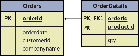
Figure 1-2 Data model after applying 2NF and before 3NF.
3NF
The third normal form also has two rules. The data must meet the second normal form. Also, all nonkey attributes must be dependent on candidate keys nontransitively. Informally, this rule means that all nonkey attributes must be mutually independent. In other words, one nonkey attribute cannot be dependent on another nonkey attribute.
The Orders and OrderDetails relations described previously now conform to the second normal form. Remember that the Orders relation at this point contains the attributes orderid, orderdate, customerid, and companyname, with the primary key defined on orderid. Both customerid and companyname depend on the whole primary key—orderid. For example, you need the entire primary key to find the customerid representing the customer who placed the order. Similarly, you need the whole primary key to find the company name of the customer who placed the order. However, customerid and companyname are also dependent on each other. To meet the third normal form, you need to add a Customers relation (shown in Figure 1-3) with the attributes customerid (as the primary key) and companyname. Then you can remove the companyname attribute from the Orders relation.
)
Figure 1-3 Data model after applying 3NF.
Informally, 2NF and 3NF are commonly summarized with the sentence, “Every non-key attribute is dependent on the key, the whole key, and nothing but the key—so help me Codd.”
There are higher normal forms beyond Codd’s original first three normal forms that involve compound primary keys and temporal databases, but they are outside the scope of this book.
NOTE
SQL, as well as T-SQL, permit violating all the normal forms in real tables. It’s the data modeler’s prerogative and responsibility to design a normalized model.
Types of database systems
Two main types of systems, or workloads, use SQL Server as their database and T-SQL to manage and manipulate the data: online transactional processing (OLTP) and data warehouses (DWs). Figure 1-4 illustrates those systems and the transformation process that usually takes place between them.
)
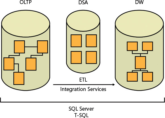
Figure 1-4 Classes of database systems.
Here’s a quick description of what each acronym represents:
OLTP: online transactional processing
DSA: data-staging area
DW: data warehouse
ETL: extract, transform, and load
Online transactional processing
Data is entered initially into an online transactional processing system. The primary focus of an OLTP system is data entry and not reporting—transactions mainly insert, update, and delete data. The relational model is targeted primarily at OLTP systems, where a normalized model provides both good performance for data entry and data consistency. In a normalized environment, each table represents a single entity and keeps redundancy to a minimum. When you need to modify a fact, you need to modify it in only one place. This results in optimized performance for data modifications and little chance for error.
However, an OLTP environment is not suitable for reporting purposes because a normalized model usually involves many tables (one for each entity) with complex relationships. Even simple reports require joining many tables, resulting in complex and poorly performing queries.
You can implement an OLTP database in SQL Server and both manage it and query it with T-SQL.
Data warehouses
A data warehouse (DW) is an environment designed for data-retrieval and reporting purposes. When it serves an entire organization, such an environment is called a data warehouse; when it serves only part of the organization (such as a specific department) or a subject matter area in the organization, it is called a data mart. The data model of a data warehouse is designed and optimized mainly to support data-retrieval needs. The model has intentional redundancy, fewer tables, and simpler relationships, ultimately resulting in simpler and more efficient queries than an OLTP environment.
The simplest data-warehouse design is called a star schema. The star schema includes several dimension tables and a fact table. Each dimension table represents a subject by which you want to analyze the data. For example, in a system that deals with orders and sales, you will probably want to analyze data by dimensions such as customers, products, employees, and time.
In a star schema, each dimension is implemented as a single table with redundant data. For example, a product dimension could be implemented as a single ProductDim table instead of three normalized tables: Products, ProductSubCategories, and ProductCategories. If you normalize a dimension table, which results in multiple tables representing that dimension, you get what’s known as a snowflake dimension. A schema that contains snowflake dimensions is known as a snowflake schema. A star schema is considered a special case of a snowflake schema.
The fact table holds the facts and measures, such as quantity and value, for each relevant combination of dimension keys. For example, for each relevant combination of customer, product, employee, and day, the fact table would have a row containing the quantity and value. Note that data in a data warehouse is typically preaggregated to a certain level of granularity (such as a day), unlike data in an OLTP environment, which is usually recorded at the transaction level.
Historically, early versions of SQL Server mainly targeted OLTP environments, but eventually SQL Server also started targeting data-warehouse systems and data-analysis needs. You can implement a data warehouse as a SQL Server database and manage and query it with T-SQL.
The process that pulls data from source systems (OLTP and others), manipulates it, and loads it into the data warehouse is called extract, transform, and load, or ETL. SQL Server provides a tool called Microsoft SQL Server Integration Services (SSIS) to handle ETL needs.
Often the ETL process will involve the use of a data-staging area (DSA) between the OLTP and the DW. The DSA usually resides in a relational database, such as a SQL Server database, and is used as the data-cleansing area. The DSA is not open to end users.